Problem Statement : Given a graph that represents a flow network where every edge has a capacity. Also given two vertices source ‘s’ and sink ‘t’ in the graph, find the maximum possible flow from s to t with the following constraints :
Flow on an edge doesn’t exceed the given capacity of the edge.
An incoming flow is equal to an outgoing flow for every vertex except s and t.
For example:
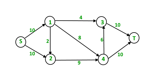
In the following input graph,
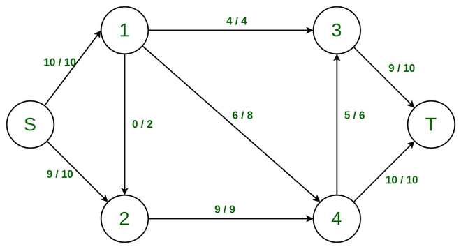
the maximum s-t flow is 19 which is shown below.
Background :
Max Flow Problem Introduction: We introduced the Maximum Flow problem, discussed Greedy Algorithm, and introduced the residual graph.
The time complexity of Edmond Karp Implementation is O(VE2). In this post, a new Dinic's algorithm is discussed which is a faster algorithm and takes O(EV2).
Like Edmond Karp's algorithm, Dinic's algorithm uses following concepts :
A flow is maximum if there is no s to t path in residual graph.
BFS is used in a loop. There is a difference though in the way we use BFS in both algorithms.
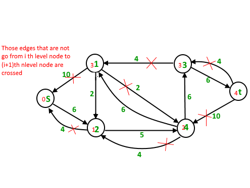
In Edmond's Karp algorithm, we use BFS to find an augmenting path and send flow across this path. In Dinic's algorithm, we use BFS to check if more flow is possible and to construct level graph. In level graph, we assign levels to all nodes, level of a node is shortest distance (in terms of number of edges) of the node from source. Once level graph is constructed, we send multiple flows using this level graph. This is the reason it works better than Edmond Karp. In Edmond Karp, we send only flow that is send across the path found by BFS.
Outline of Dinic's algorithm :
Initialize residual graph G as given graph.
Do BFS of G to construct a level graph (or assign levels to vertices) and also check if more flow is possible.
If more flow is not possible, then return
Send multiple flows in G using level graph until blocking flow is reached. Here using level graph means, in every flow, levels of path nodes should be 0, 1, 2...(in order) from s to t.
A flow is Blocking Flow if no more flow can be sent using level graph, i.e., no more s-t path exists such that path vertices have current levels 0, 1, 2... in order. Blocking Flow can be seen same as maximum flow path in Greedy algorithm discussed here.
Illustration : Initial Residual Graph (Same as given Graph)
Total Flow = 0
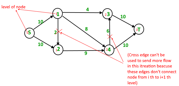
First Iteration : We assign levels to all nodes using BFS. We also check if more flow is possible (or there is a s-t path in residual graph).
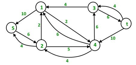
Now we find blocking flow using levels (means every flow path should have levels as 0, 1, 2, 3). We send three flows together. This is where it is optimized compared to Edmond Karp where we send one flow at a time. 4 units of flow on path s - 1 - 3 - t. 6 units of flow on path s - 1 - 4 - t. 4 units of flow on path s - 2 - 4 - t. Total flow = Total flow + 4 + 6 + 4 = 14 After one iteration, residual graph changes to following.
Second Iteration : We assign new levels to all nodes using BFS of above modified residual graph. We also check if more flow is possible (or there is a s-t path in residual graph).
Now we find blocking flow using levels (means every flow path should have levels as 0, 1, 2, 3, 4). We can send only one flow this time. 5 units of flow on path s - 2 - 4 - 3 - t Total flow = Total flow + 5 = 19 The new residual graph is
Third Iteration : We run BFS and create a level graph. We also check if more flow is possible and proceed only if possible. This time there is no s-t path in residual graph, so we terminate the algorithm.
Implementation : Below is c++ implementation of Dinic's algorithm:
CPP
// C++ implementation of Dinic's Algorithm#include<bits/stdc++.h>usingnamespacestd;// A structure to represent a edge between// two vertexstructEdge{intv;// Vertex v (or "to" vertex)// of a directed edge u-v. "From"// vertex u can be obtained using// index in adjacent array.intflow;// flow of data in edgeintC;// capacityintrev;// To store index of reverse// edge in adjacency list so that// we can quickly find it.};// Residual GraphclassGraph{intV;// number of vertexint*level;// stores level of a nodevector<Edge>*adj;public:Graph(intV){adj=newvector<Edge>[V];this->V=V;level=newint[V];}// add edge to the graphvoidaddEdge(intu,intv,intC){// Forward edge : 0 flow and C capacityEdgea{v,0,C,(int)adj[v].size()};// Back edge : 0 flow and 0 capacityEdgeb{u,0,0,(int)adj[u].size()};adj[u].push_back(a);adj[v].push_back(b);// reverse edge}boolBFS(ints,intt);intsendFlow(ints,intflow,intt,intptr[]);intDinicMaxflow(ints,intt);};// Finds if more flow can be sent from s to t.// Also assigns levels to nodes.boolGraph::BFS(ints,intt){for(inti=0;i<V;i++)level[i]=-1;level[s]=0;// Level of source vertex// Create a queue, enqueue source vertex// and mark source vertex as visited here// level[] array works as visited array also.list<int>q;q.push_back(s);vector<Edge>::iteratori;while(!q.empty()){intu=q.front();q.pop_front();for(i=adj[u].begin();i!=adj[u].end();i++){Edge&e=*i;if(level[e.v]<0&&e.flow<e.C){// Level of current vertex is,// level of parent + 1level[e.v]=level[u]+1;q.push_back(e.v);}}}// IF we can not reach to the sink we// return false else truereturnlevel[t]<0?false:true;}// A DFS based function to send flow after BFS has// figured out that there is a possible flow and// constructed levels. This function called multiple// times for a single call of BFS.// flow : Current flow send by parent function call// start[] : To keep track of next edge to be explored.// start[i] stores count of edges explored// from i.// u : Current vertex// t : SinkintGraph::sendFlow(intu,intflow,intt,intstart[]){// Sink reachedif(u==t)returnflow;// Traverse all adjacent edges one -by - one.for(;start[u]<adj[u].size();start[u]++){// Pick next edge from adjacency list of uEdge&e=adj[u][start[u]];if(level[e.v]==level[u]+1&&e.flow<e.C){// find minimum flow from u to tintcurr_flow=min(flow,e.C-e.flow);inttemp_flow=sendFlow(e.v,curr_flow,t,start);// flow is greater than zeroif(temp_flow>0){// add flow to current edgee.flow+=temp_flow;// subtract flow from reverse edge// of current edgeadj[e.v][e.rev].flow-=temp_flow;returntemp_flow;}}}return0;}// Returns maximum flow in graphintGraph::DinicMaxflow(ints,intt){// Corner caseif(s==t)return-1;inttotal=0;// Initialize result// Augment the flow while there is path// from source to sinkwhile(BFS(s,t)==true){// store how many edges are visited// from V { 0 to V }int*start=newint[V+1]{0};// while flow is not zero in graph from S to Dwhile(intflow=sendFlow(s,INT_MAX,t,start)){// Add path flow to overall flowtotal+=flow;}// Remove allocated arraydelete[]start;}// return maximum flowreturntotal;}// Driver Codeintmain(){Graphg(6);g.addEdge(0,1,16);g.addEdge(0,2,13);g.addEdge(1,2,10);g.addEdge(1,3,12);g.addEdge(2,1,4);g.addEdge(2,4,14);g.addEdge(3,2,9);g.addEdge(3,5,20);g.addEdge(4,3,7);g.addEdge(4,5,4);// next exmp/*g.addEdge(0, 1, 3 ); g.addEdge(0, 2, 7 ) ; g.addEdge(1, 3, 9); g.addEdge(1, 4, 9 ); g.addEdge(2, 1, 9 ); g.addEdge(2, 4, 9); g.addEdge(2, 5, 4); g.addEdge(3, 5, 3); g.addEdge(4, 5, 7 ); g.addEdge(0, 4, 10); // next exp g.addEdge(0, 1, 10); g.addEdge(0, 2, 10); g.addEdge(1, 3, 4 ); g.addEdge(1, 4, 8 ); g.addEdge(1, 2, 2 ); g.addEdge(2, 4, 9 ); g.addEdge(3, 5, 10 ); g.addEdge(4, 3, 6 ); g.addEdge(4, 5, 10 ); */cout<<"Maximum flow "<<g.DinicMaxflow(0,5);return0;}
Java
// JAVA implementation of above approachimportjava.util.*;classEdge{publicintv;// Vertex v (or "to" vertex)// of a directed edge u-v. "From"// vertex u can be obtained using// index in adjacent arraypublicintflow;// flow of data in edgepublicintC;// Capacitypublicintrev;// To store index of reverse// edge in adjacency list so that// we can quickly find it.publicEdge(intv,intflow,intC,intrev){this.v=v;this.flow=flow;this.C=C;this.rev=rev;}}// Residual GraphclassGraph{privateintV;// No. of vertexprivateint[]level;// Stores level of graphprivateList<Edge>[]adj;publicGraph(intV){adj=newArrayList[V];for(inti=0;i<V;i++){adj[i]=newArrayList<Edge>();}this.V=V;level=newint[V];}// Add edge to the graphpublicvoidaddEdge(intu,intv,intC){// Forward edge : 0 flow and C capacityEdgea=newEdge(v,0,C,adj[v].size());// Back edge : 0 flow and 0 capacityEdgeb=newEdge(u,0,0,adj[u].size());adj[u].add(a);adj[v].add(b);}// Finds if more flow can be sent from s to t.// Also assigns levels to nodes.publicbooleanBFS(ints,intt){for(inti=0;i<V;i++){level[i]=-1;}level[s]=0;// Level of source vertex// Create a queue, enqueue source vertex// and mark source vertex as visited here// level[] array works as visited array also.LinkedList<Integer>q=newLinkedList<Integer>();q.add(s);ListIterator<Edge>i;while(q.size()!=0){intu=q.poll();for(i=adj[u].listIterator();i.hasNext();){Edgee=i.next();if(level[e.v]<0&&e.flow<e.C){// Level of current vertex is -// Level of parent + 1level[e.v]=level[u]+1;q.add(e.v);}}}returnlevel[t]<0?false:true;}// A DFS based function to send flow after BFS has// figured out that there is a possible flow and// constructed levels. This function called multiple// times for a single call of BFS.// flow : Current flow send by parent function call// start[] : To keep track of next edge to be explored.// start[i] stores count of edges explored// from i.// u : Current vertex// t : SinkpublicintsendFlow(intu,intflow,intt,intstart[]){// Sink reachedif(u==t){returnflow;}// Traverse all adjacent edges one -by - one.for(;start[u]<adj[u].size();start[u]++){// Pick next edge from adjacency list of uEdgee=adj[u].get(start[u]);if(level[e.v]==level[u]+1&&e.flow<e.C){// find minimum flow from u to tintcurr_flow=Math.min(flow,e.C-e.flow);inttemp_flow=sendFlow(e.v,curr_flow,t,start);// flow is greater than zeroif(temp_flow>0){// add flow to current edgee.flow+=temp_flow;// subtract flow from reverse edge// of current edgeadj[e.v].get(e.rev).flow-=temp_flow;returntemp_flow;}}}return0;}// Returns maximum flow in graphpublicintDinicMaxflow(ints,intt){if(s==t){return-1;}inttotal=0;// Augment the flow while there is path// from source to sinkwhile(BFS(s,t)==true){// store how many edges are visited// from V { 0 to V }int[]start=newint[V+1];// while flow is not zero in graph from S to Dwhile(true){intflow=sendFlow(s,Integer.MAX_VALUE,t,start);if(flow==0){break;}// Add path flow to overall flowtotal+=flow;}}// Return maximum flowreturntotal;}}// Driver CodepublicclassMain{publicstaticvoidmain(Stringargs[]){Graphg=newGraph(6);g.addEdge(0,1,16);g.addEdge(0,2,13);g.addEdge(1,2,10);g.addEdge(1,3,12);g.addEdge(2,1,4);g.addEdge(2,4,14);g.addEdge(3,2,9);g.addEdge(3,5,20);g.addEdge(4,3,7);g.addEdge(4,5,4);// next exmp/*g.addEdge(0, 1, 3 ); g.addEdge(0, 2, 7 ) ; g.addEdge(1, 3, 9); g.addEdge(1, 4, 9 ); g.addEdge(2, 1, 9 ); g.addEdge(2, 4, 9); g.addEdge(2, 5, 4); g.addEdge(3, 5, 3); g.addEdge(4, 5, 7 ); g.addEdge(0, 4, 10); // next exp g.addEdge(0, 1, 10); g.addEdge(0, 2, 10); g.addEdge(1, 3, 4 ); g.addEdge(1, 4, 8 ); g.addEdge(1, 2, 2 ); g.addEdge(2, 4, 9 ); g.addEdge(3, 5, 10 ); g.addEdge(4, 3, 6 ); g.addEdge(4, 5, 10 ); */System.out.println("Maximum flow "+g.DinicMaxflow(0,5));}}// This code is contributed by Amit Mangal
Python3
# Python implementation of Dinic's AlgorithmclassEdge:def__init__(self,v,flow,C,rev):self.v=vself.flow=flowself.C=Cself.rev=rev# Residual GraphclassGraph:def__init__(self,V):self.adj=[[]foriinrange(V)]self.V=Vself.level=[0foriinrange(V)]# add edge to the graphdefaddEdge(self,u,v,C):# Forward edge : 0 flow and C capacitya=Edge(v,0,C,len(self.adj[v]))# Back edge : 0 flow and 0 capacityb=Edge(u,0,0,len(self.adj[u]))self.adj[u].append(a)self.adj[v].append(b)# Finds if more flow can be sent from s to t# Also assigns levels to nodesdefBFS(self,s,t):foriinrange(self.V):self.level[i]=-1# Level of source vertexself.level[s]=0# Create a queue, enqueue source vertex# and mark source vertex as visited here# level[] array works as visited array alsoq=[]q.append(s)whileq:u=q.pop(0)foriinrange(len(self.adj[u])):e=self.adj[u][i]ifself.level[e.v]<0ande.flow<e.C:# Level of current vertex is# level of parent + 1self.level[e.v]=self.level[u]+1q.append(e.v)# If we can not reach to the sink we# return False else TruereturnFalseifself.level[t]<0elseTrue# A DFS based function to send flow after BFS has# figured out that there is a possible flow and# constructed levels. This functions called multiple# times for a single call of BFS.# flow : Current flow send by parent function call# start[] : To keep track of next edge to be explored# start[i] stores count of edges explored# from i# u : Current vertex# t : SinkdefsendFlow(self,u,flow,t,start):# Sink reachedifu==t:returnflow# Traverse all adjacent edges one -by -onewhilestart[u]<len(self.adj[u]):# Pick next edge from adjacency list of ue=self.adj[u][start[u]]ifself.level[e.v]==self.level[u]+1ande.flow<e.C:# find minimum flow from u to tcurr_flow=min(flow,e.C-e.flow)temp_flow=self.sendFlow(e.v,curr_flow,t,start)# flow is greater than zeroiftemp_flowandtemp_flow>0:# add flow to current edgee.flow+=temp_flow# subtract flow from reverse edge# of current edgeself.adj[e.v][e.rev].flow-=temp_flowreturntemp_flowstart[u]+=1# Returns maximum flow in graphdefDinicMaxflow(self,s,t):# Corner caseifs==t:return-1# Initialize resulttotal=0# Augument the flow while there is path# from source to sinkwhileself.BFS(s,t)==True:# store how many edges are visited# from V { 0 to V }start=[0foriinrange(self.V+1)]whileTrue:flow=self.sendFlow(s,float('inf'),t,start)ifnotflow:break# Add path flow to overall flowtotal+=flow# return maximum flowreturntotalg=Graph(6)g.addEdge(0,1,16)g.addEdge(0,2,13)g.addEdge(1,2,10)g.addEdge(1,3,12)g.addEdge(2,1,4)g.addEdge(2,4,14)g.addEdge(3,2,9)g.addEdge(3,5,20)g.addEdge(4,3,7)g.addEdge(4,5,4)print("Maximum flow",g.DinicMaxflow(0,5))# This code is contributed by rupasriachanta421.
C#
usingSystem;usingSystem.Collections.Generic;classEdge{publicintv;// Vertex v (or "to" vertex)// of a directed edge u-v. "From"// vertex u can be obtained using// index in adjacent arraypublicintflow;// flow of data in edgepublicintC;// capacitypublicintrev;// To store index of reverse// edge in adjacency list so that// we can quickly find it.publicEdge(intv,intflow,intC,intrev){this.v=v;this.flow=flow;this.C=C;this.rev=rev;}}// Residual GraphclassGraph{privateintV;// No. of vertex privateint[]level;// Stores level of graph privateList<Edge>[]adj;publicGraph(intV){adj=newList<Edge>[V];for(inti=0;i<V;i++){adj[i]=newList<Edge>();}this.V=V;level=newint[V];}// Add edge to the graphpublicvoidaddEdge(intu,intv,intC){// Forward edge : 0 flow and C capacityEdgea=newEdge(v,0,C,adj[v].Count);// Back edge : 0 flow and 0 capacityEdgeb=newEdge(u,0,0,adj[u].Count);adj[u].Add(a);adj[v].Add(b);}// Finds if more flow can be sent from s to t.// Also assigns levels to nodes.publicboolBFS(ints,intt){for(intj=0;j<V;j++){level[j]=-1;}level[s]=0;// Level of source vertex// Create a queue, enqueue source vertex// and mark source vertex as visited here// level[] array works as visited array also.Queue<int>q=newQueue<int>();q.Enqueue(s);List<Edge>.Enumeratori;while(q.Count!=0){intu=q.Dequeue();for(i=adj[u].GetEnumerator();i.MoveNext();){Edgee=i.Current;if(level[e.v]<0&&e.flow<e.C){// Level of current vertex is -// Level of parent + 1level[e.v]=level[u]+1;q.Enqueue(e.v);}}}returnlevel[t]<0?false:true;}// A DFS based function to send flow after BFS has// figured out that there is a possible flow and// constructed levels. This function called multiple// times for a single call of BFS.// flow : Current flow send by parent function call// start[] : To keep track of next edge to be explored.// start[i] stores count of edges explored// from i.// u : Current vertex// t : SinkpublicintsendFlow(intu,intflow,intt,int[]start){// Sink reachedif(u==t){returnflow;}// Traverse all adjacent edges one -by - one.for(;start[u]<adj[u].Count;start[u]++){// Pick next edge from adjacency list of uEdgee=adj[u][start[u]];if(level[e.v]==level[u]+1&&e.flow<e.C){// find minimum flow from u to tintcurr_flow=Math.Min(flow,e.C-e.flow);inttemp_flow=sendFlow(e.v,curr_flow,t,start);// flow is greater than zeroif(temp_flow>0){// add flow to current edgee.flow+=temp_flow;// subtract flow from reverse edge// of current edgeadj[e.v][e.rev].flow-=temp_flow;returntemp_flow;}}}return0;}// Returns maximum flow in graphpublicintDinicMaxflow(ints,intt){if(s==t){return-1;}inttotal=0;// Augment the flow while there is path// from source to sinkwhile(BFS(s,t)==true){// store how many edges are visited// from V { 0 to V }int[]start=newint[V+1];// while flow is not zero in graph from S to Dwhile(true){intflow=sendFlow(s,int.MaxValue,t,start);if(flow==0){break;}// Add path flow to overall flowtotal+=flow;}}// Return maximum flowreturntotal;}}// Driver CodepublicclassGfg{publicstaticvoidMain(){Graphg=newGraph(6);g.addEdge(0,1,16);g.addEdge(0,2,13);g.addEdge(1,2,10);g.addEdge(1,3,12);g.addEdge(2,1,4);g.addEdge(2,4,14);g.addEdge(3,2,9);g.addEdge(3,5,20);g.addEdge(4,3,7);g.addEdge(4,5,4);// next exmp/*g.addEdge(0, 1, 3 ); g.addEdge(0, 2, 7 ) ; g.addEdge(1, 3, 9); g.addEdge(1, 4, 9 ); g.addEdge(2, 1, 9 ); g.addEdge(2, 4, 9); g.addEdge(2, 5, 4); g.addEdge(3, 5, 3); g.addEdge(4, 5, 7 ); g.addEdge(0, 4, 10); // next exp g.addEdge(0, 1, 10); g.addEdge(0, 2, 10); g.addEdge(1, 3, 4 ); g.addEdge(1, 4, 8 ); g.addEdge(1, 2, 2 ); g.addEdge(2, 4, 9 ); g.addEdge(3, 5, 10 ); g.addEdge(4, 3, 6 ); g.addEdge(4, 5, 10 ); */Console.Write("Maximum flow "+g.DinicMaxflow(0,5));}}
JavaScript
// Javascript implementation of Dinic's Algorithm// A class to represent a edge between// two vertexclassEdge{constructor(v,flow,C,rev){// Vertex v (or "to" vertex)// of a directed edge u-v. "From"// vertex u can be obtained using// index in adjacent array.this.v=v;// flow of data in edgethis.flow=flow;// capacitythis.C=C;// To store index of reverse// edge in adjacency list so that// we can quickly find it.this.rev=rev;}}// Residual GraphclassGraph{constructor(V){this.V=V;// number of vertexthis.adj=Array.from(Array(V),()=>newArray());this.level=newArray(V);// stores level of a node}// add edge to the graphaddEdge(u,v,C){// Forward edge : 0 flow and C capacityleta=newEdge(v,0,C,this.adj[v].length);// Back edge : 0 flow and 0 capacityletb=newEdge(u,0,0,this.adj[u].length);this.adj[u].push(a);this.adj[v].push(b);// reverse edge}// Finds if more flow can be sent from s to t.// Also assigns levels to nodes.BFS(s,t){for(leti=0;i<this.V;i++)this.level[i]=-1;this.level[s]=0;// Level of source vertex// Create a queue, enqueue source vertex// and mark source vertex as visited here// level[] array works as visited array also.letq=newArray();q.push(s);while(q.length!=0){letu=q[0];q.shift();for(letjinthis.adj[u]){lete=this.adj[u][j];if(this.level[e.v]<0&&e.flow<e.C){// Level of current vertex is,// level of parent + 1this.level[e.v]=this.level[u]+1;q.push(e.v);}}}// IF we can not reach to the sink we// return false else truereturnthis.level[t]<0?false:true;}// A DFS based function to send flow after BFS has// figured out that there is a possible flow and// constructed levels. This function called multiple// times for a single call of BFS.// flow : Current flow send by parent function call// start[] : To keep track of next edge to be explored.// start[i] stores count of edges explored// from i.// u : Current vertex// t : SinksendFlow(u,flow,t,start){// Sink reachedif(u==t)returnflow;// Traverse all adjacent edges one -by - one.while(start[u]<this.adj[u].length){// Pick next edge from adjacency list of ulete=this.adj[u][start[u]];if(this.level[e.v]==this.level[u]+1&&e.flow<e.C){// find minimum flow from u to tletcurr_flow=Math.min(flow,e.C-e.flow);lettemp_flow=this.sendFlow(e.v,curr_flow,t,start);// flow is greater than zeroif(temp_flow>0){// add flow to current edgee.flow+=temp_flow;// subtract flow from reverse edge// of current edgethis.adj[e.v][e.rev].flow-=temp_flow;returntemp_flow;}}start[u]=start[u]+1;}return0;}// Returns maximum flow in graphDinicMaxflow(s,t){// Corner caseif(s==t)return-1;lettotal=0;// Initialize result// Augment the flow while there is path// from source to sinkwhile(this.BFS(s,t)==true){// store how many edges are visited// from V { 0 to V }letstart=newArray(this.V+1);start.fill(0);// while flow is not zero in graph from S to Dwhile(true){letflow=this.sendFlow(s,Number.MAX_VALUE,t,start);if(!flow){break;}// Add path flow to overall flowtotal+=flow;}}// return maximum flowreturntotal;}}// Driver Codeletg=newGraph(6);g.addEdge(0,1,16);g.addEdge(0,2,13);g.addEdge(1,2,10);g.addEdge(1,3,12);g.addEdge(2,1,4);g.addEdge(2,4,14);g.addEdge(3,2,9);g.addEdge(3,5,20);g.addEdge(4,3,7);g.addEdge(4,5,4);// next exmp/*g.addEdge(0, 1, 3 ); g.addEdge(0, 2, 7 ) ; g.addEdge(1, 3, 9); g.addEdge(1, 4, 9 ); g.addEdge(2, 1, 9 ); g.addEdge(2, 4, 9); g.addEdge(2, 5, 4); g.addEdge(3, 5, 3); g.addEdge(4, 5, 7 ); g.addEdge(0, 4, 10); // next exp g.addEdge(0, 1, 10); g.addEdge(0, 2, 10); g.addEdge(1, 3, 4 ); g.addEdge(1, 4, 8 ); g.addEdge(1, 2, 2 ); g.addEdge(2, 4, 9 ); g.addEdge(3, 5, 10 ); g.addEdge(4, 3, 6 ); g.addEdge(4, 5, 10 ); */console.log("Maximum flow "+g.DinicMaxflow(0,5));
Output
Maximum flow 23
Time Complexity : O(EV2).
Doing a BFS to construct level graph takes O(E) time.
Sending multiple more flows until a blocking flow is reached takes O(VE) time.
The outer loop runs at-most O(V) time.
In each iteration, we construct new level graph and find blocking flow. It can be proved that the number of levels increase at least by one in every iteration (Refer the below reference video for the proof). So the outer loop runs at most O(V) times.
Therefore overall time complexity is O(EV2).
Space complexity: The space complexity of Dinic’s algorithm is O(V+E), since it requires O(V) to store the level array and O(E) to store the graph's adjacency list.
We use cookies to ensure you have the best browsing experience on our website. By using our site, you
acknowledge that you have read and understood our
Cookie Policy &
Privacy Policy
Improvement
Suggest Changes
Help us improve. Share your suggestions to enhance the article. Contribute your expertise and make a difference in the GeeksforGeeks portal.
Create Improvement
Enhance the article with your expertise. Contribute to the GeeksforGeeks community and help create better learning resources for all.