


ABSTRACT
Using imaging data from the Solar TErrestrial RElations Observatory (STEREO) mission, we empirically reconstruct the time-dependent three-dimensional morphology of a coronal mass ejection (CME) from 2008 June 1, which exhibits significant variation in shape as it travels from the Sun to 1
Export citation and abstract BibTeX RIS
1. INTRODUCTION
The primary goal of the Solar TErrestrial RElations Observatory (STEREO) mission (Kaiser et al. 2008) is to improve our understanding of the three-dimensional (3D) morphology of coronal mass ejections (CMEs). The deep, extended solar minimum of 2008–09 did not provide many dramatic CMEs for the two STEREO spacecraft to study, but on 2008 June 1, a very slow CME is observed drifting slowly away from the Sun, with the event clearly discernible in images from both spacecraft. The CME expands off the east limb as viewed from STEREO-A, which at the time was located 25° ahead of the Earth in its orbit around the Sun. In contrast, the CME appears as a halo event from the perspective of STEREO-B, orbiting 29° behind the Earth.
The imagers that make up the SECCHI instrument packages on each STEREO spacecraft (Howard et al. 2008) successfully track this CME continuously from close to the Sun to 1
One final factor that has made this event worthy of study is the lack of any discernable surface activity associated with it. Both the in situ detection at STEREO-B and the eastward direction of the CME in STEREO-A images demonstrate that the halo appearance of the CME seen from STEREO-B's perspective is due to a front-side event and not a backside event. Nevertheless, the EUVI imagers on both STEREO spacecraft, which view the solar corona in various EUV bandpasses, detect no flaring or filament eruption at the time of the CME's inception (Robbrecht et al. 2009), demonstrating more clearly than ever before that CME initiation does not necessarily require any obvious surface driver, at least for the very slow "streamer blowout" CME class to which this event clearly belongs (Howard et al. 1985). The purpose of this paper is to study the morphological and kinematic evolution of this CME, from its inception to its arrival at STEREO-B, based on an empirical analysis of STEREO images of the event from both the A and B spacecraft.
2. MORPHOLOGY OF THE JUNE 1 CME: QUALITATIVE ASSESSMENT
Each STEREO spacecraft carries four white-light telescopes that can observe CMEs at different distances from the Sun (Howard et al. 2008). There are two coronagraphs, COR1 and COR2, that observe the Sun's white-light corona at angular distances from Sun-center of 0 37–107 and 07–42, respectively, corresponding to distances in the plane of the sky of 1.4–4.0 R☉ for COR1 and 2.5–15.6 R☉ for COR2. And there are two heliospheric imagers, HI1 and HI2, that monitor the interplanetary medium (IPM) in between the Sun and Earth, where HI1 observes elongation angles from Sun-center of 39–241 and HI2 observes from 19°–89°.
Figure 1 shows four STEREO images of the 2008 June 1 event. This CME is a halo event from STEREO-B's perspective. While apparent in COR2-B movies, the halo is quite faint in the static COR2-B image in Figure 1, so an outline is provided to guide the eye. In COR2-A, the CME has a compact appearance with a vaguely circular top. Such a semblance is commonly seen for CMEs and is often interpreted as representing the apex of a flux rope viewed edge-on (Chen et al. 1997; Wood et al. 1999; Low 2001; Cremades & Bothmer 2004; Krall 2007). However, the HI1-A appearance of the June 1 CME is very different, looking more like a broad flux rope viewed closer to face-on. This visage is more consistent with the flux rope orientation that Möstl et al. (2009) infer for the CME based on the in situ observations from STEREO-B. They estimate a −45° tilt of the flux rope relative to the ecliptic plane and argue that this is consistent with the HI1-A and HI2-A appearance of the CME. The suggestion is made that perhaps the change in appearance between COR2-A and HI1-A is due to a ∼45° clockwise rotation of the flux rope.
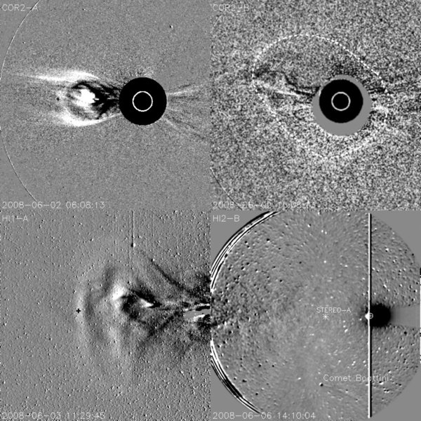
Figure 1. Four sample images of the 2008 June 1 CME, the left two from STEREO-A and the right two from STEREO-B. Note the dramatic change in CME appearance between the COR2-A and HI1-A images. The CME is a faint halo event from the perspective of STEREO-B, and a dotted line is used to mark the faint halo's location in the COR2-B image. The HI2-B image shows the broad, and very faint CME front hitting Comet Boattini, affecting the behavior of the comet's tail. The positions of Earth and STEREO-A are also indicated in the HI2-B image.
Download figure:
Standard image High-resolution imageAlthough a rotation may be consistent with STEREO-A's view of the event, it is questionable whether it is the best interpretation of STEREO-B's images. To us, the shape of the COR2-B halo is already suggestive of a roughly −45° tilt of the CME at early times. Furthermore, we see no evidence for any clockwise rotational motion of the halo in COR1-B, COR2-B, or HI1-B movies. Thus, our preferred interpretation of the event is that the CME flux rope possesses a tilt right from the start, but this orientation is not evident at early times due to the flux rope being initially very fat, making the tilt angle difficult to infer from STEREO-A's perspective. In this paradigm, which will be presented in detail in Section 4, the change in appearance between COR2-A and HI1-A is due to a narrowing of the flux rope and a flattening of its top with time, as the CME moves outward from the Sun.
Finally, there is a comet visible in the HI2-B image in Figure 1, which is struck by the CME. This is Comet C/2007 W1 Boattini. STEREO has previously observed other comets interacting with the solar wind and transients within it (Vourlidas et al. 2007; Jia et al. 2009). There is little evidence of a tail for Comet Boattini during the day leading up to the CME's passage over the comet, at least not in the HI2-B images, but a tail appears and brightens starting at about 4:10 UT on June 6. The tail then experiences a clear disconnection event at about 8:10 UT and remains active and variable for about 2 days thereafter before fading again. If we associate the disconnection event at June 6, 8:10 UT with the timing of the CME's primary density pulse hitting the comet, we can use our knowledge of the comet's orbit to pinpoint the CME's location at 8:10 UT, at least at one point along the CME front. In this way, the comet provides a useful constraint for our morphological modeling. In heliocentric Earth ecliptic (HEE) coordinates, the comet's position at the time of CME impact is (x, y, z) = (0.898, −0.096, −0.157)
3. KINEMATICS OF THE JUNE 1 CME
Measuring CME velocities and trajectories is crucial for understanding how CMEs propagate through the IPM. It is also important for space weather forecasting purposes in order to accurately predict if and when a CME will hit Earth. For our purposes, we need a kinematic model of the June 1 CME to properly scale our time-dependent 3D morphological models. Both kinematic and morphological understanding of the event are necessary to generate synthetic images that can be compared directly with the real images, providing the ultimate test of both the kinematic and morphological aspects of the analysis.
It is much easier to measure a CME's radial motion from the Sun when the CME is observed from the side than if the CME is moving directly toward or away from an observer. This means that for the June 1 CME STEREO-A is in a much more useful location for a kinematic analysis than STEREO-B. We measure the elongation angle of the CME as a function of time from all STEREO-A images of the event, from COR1-A all the way through HI2-A. In the COR2-A and HI1-A panels of Figure 1, plus signs indicate how we have marked the leading edge of the CME.
A kinematic analysis requires computing real distances, r, from the measured elongation angles,  . There are two simple methods that have been used in the past, the "point-P" and "fixed-ϕ" methods (Kahler & Webb 2007; Howard et al. 2007, 2008; Sheeley et al. 2008; Wood et al. 2009a). The former assumes an extremely broad spherical front centered on the Sun, with

where d is the distance from the observer to the Sun, the observer being STEREO-A in this case. The latter assumes a very narrow CME, with
where ϕ is the angle between the CME trajectory and the observer's line of sight to the Sun. More recently, Lugaz et al. (2009) have proposed a third method, which approximates the CME as a sphere centered halfway between the Sun and the CME's leading edge. This assumption yields
Lugaz et al. (2009) call this the "harmonic mean" approximation, since an r value computed under this assumption represents the intermediate harmonic mean of values computed under the other two approximations.
The top panel of Figure 2 shows the leading edge distances computed for the June 1 CME for all three approximations, and the bottom panel shows the inferred velocity of the CME's leading edge. The morphological analysis presented in Section 4 suggests a CME trajectory of ϕ = 63°, so that is what is assumed for the fixed-ϕ and harmonic mean assumptions. Velocities are generally computed from adjacent distance data points, but this sometimes leads to velocities with huge error bars, which vary wildly in time in a very misleading fashion. For this reason, as we compute the velocities from left to right in the figure we actually skip distance points until the uncertainty in the computed velocity ends up under some assumed threshold value (100 km s−1 in this case), similar to what we have done in the past (Wood et al. 1999, 2009a). The velocity uncertainties are computed assuming the following estimates for the uncertainties in the distance measurements: 1% fractional errors for the COR1 and COR2 distances, and 2% and 3% uncertainties for HI1 and HI2, respectively.
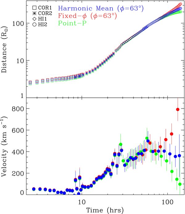
Figure 2. Distance and velocity measurements for the 2008 June 1 CME's leading edge, for three different approaches to extracting distances from elongation angle measurements. The "fixed-ϕ" method yields an implausible acceleration near 1
Download figure:
Standard image High-resolution imageThe three velocity profiles in Figure 2 are consistent throughout the COR1, COR2, and HI1 fields of view, suggesting a CME that drifts through COR1-A at a roughly constant speed of about 50 km s−1 and then accelerates through COR2-A into HI1-A, reaching a velocity of about 400 km s−1. However, the three assumptions represented by Equations (1)–(3) result in wildly different conclusions about what happens to the CME in the HI2-A field of view. The point-P approximation implies a dramatic deceleration in HI2-A, while the fixed-ϕ approximation implies a dramatic acceleration. It is very difficult to imagine any physical reason why this CME would do either this far from the Sun. The harmonic mean approximation yields a far more plausible kinematic profile, with the CME speed simply leveling off nicely at 400 km s−1.
Aside from plausibility arguments, another way to validate the harmonic mean approximation's distance and velocity measurements is to compare them with the in situ measurements of the CME by STEREO-B (see Möstl et al. 2009). We find that the CME arrival time at STEREO-B suggested by the harmonic mean measurements is within an hour of the observed June 6, UT 21:00 arrival time of the CME's main density peak. The 1
We have analyzed the kinematics of several CMEs in the past for which the fixed-ϕ approximation did not lead to implausible velocity profiles, and which accurately predicted 1
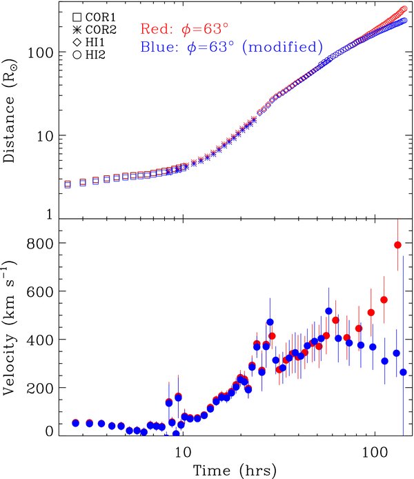
Figure 3 shows distance and velocity-versus-time computations for the June 1 CME assuming two different ϕ values, under the fixed-ϕ assumption. We already noted in Figure 2 that the ϕ = 63° fixed-ϕ model yields an improbable HI2-A acceleration and that this can be solved by switching to the harmonic mean approach. Figure 3 shows that another solution is to reduce ϕ by only 13° to ϕ = 50°. One approach to any kinematic analysis is to actually assume that the correct trajectory is whatever ϕ leads to a constant velocity far from the Sun, in effect assuming that the CME has reached some sort of terminal velocity by the time it reaches the HI2 field of view (Sheeley et al. 2008; Rouillard et al 2008). However, we would argue that for this CME the trajectory estimates close to the Sun are quite robust. Our preferred ϕ = 63° comes from our own morphological analysis in Section 4, but this result is quite consistent with the ϕ = 66° value that Thernisien et al. (2009) infer from COR2 data alone. It is also consistent with other assessments close to the Sun, which are summarized by Möstl et al. (2009).
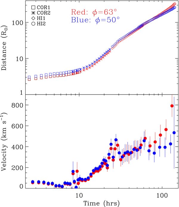
Figure 3. Distance and velocity measurements for the 2008 June 1 CME's leading edge computed under the "fixed-ϕ" approximation, assuming two different trajectory angles (ϕ). The implausible acceleration far from the Sun seen assuming ϕ = 63° can be removed by decreasing the trajectory angle to ϕ = 50°, though this angle is inconsistent with the morphological analysis.
Download figure:
Standard image High-resolution imageIs it possible that the CME trajectory actually changes from ϕ ≈ 63° close to the Sun to ϕ ≈ 50° in the HI2 field of view? In some sense, we believe that this is indeed what is happening. However, it is not that the CME is changing direction, it is instead that the part of the CME front seen as the leading edge is changing as the CME moves outward. A fundamental problem with the fixed-ϕ approach is that it assumes that a fixed observer sees the same part of the CME front as the leading edge at all times. The two panels of Figure 4 illustrate how this can be a problem. In the first panel, it is the far side of the CME front that is seen as the leading edge. This apparent leading edge shifts to the foreground side of the CME front as the CME moves outward. We believe this is why the HI2-A data seem to suggest a lower trajectory angle than our preferred ϕ = 63° angle. The part of the CME front that is being followed in HI2-A truly is at a lower trajectory angle than the actual center of the CME.
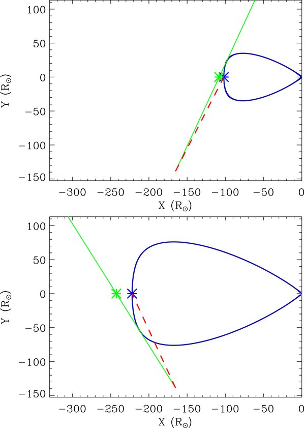
Figure 4. Demonstration of how the part of a CME front seen as the apparent leading edge can change as the CME expands. The dashed red line connects the observer to the true leading edge of the schematic CME front. The green line connects the observer to the apparent leading edge, with the green asterisk indicating where the observer will think the leading edge is based on the "fixed-ϕ" approximation. The apparent leading edge moves from the far side of the CME front in the top panel to the near side in the bottom panel.
Download figure:
Standard image High-resolution imageThe point-P and harmonic mean approximations both allow the apparent leading edge of the CME to shift along the CME front, albeit with specific assumptions about the shape of the front. For this particular CME, the allowances provided by the harmonic mean assumption seem to have led to a proper reproduction of the actual CME kinematic behavior. However, none of the three techniques represented by Equations (1)–(3) should be considered superior. Each technique will be applicable for particular viewing geometries and certain CME shapes (e.g., Howard & Tappin 2009). The fixed-ϕ approach will be best for narrow CMEs, or cases in which only a small part of a broad CME front is visible. The point-P and harmonic mean approximations will be more applicable for broad, bright CME fronts, with the point-P approximation probably being better for CMEs directed more toward the observer. A plot like Figure 2 should be helpful in assessing which technique is best for a given event, especially if the assumption is made that the best kinematic model is that which yields the flattest velocity profile far from the Sun. If the CME hits a spacecraft, the arrival time information provided by in situ data will also be helpful.
In Figure 5, we have fitted a kinematic model to the harmonic mean distance-versus-time data points from Figure 2. This is a three-phase model, somewhat analogous to kinematic models we have used to model CMEs in the past (Wood et al. 2009a, 2009b), but with differences associated with the very slow initial speed of the CME. The model assumes an initial phase of constant velocity, V1, ending at some time t1; a second phase of constant acceleration, a2, ending at some time t2; followed by a final phase of constant velocity. In addition to these four free parameters, there is a fifth involving a time shift from the model time vector to that of the actual measurements. Figure 5 shows the best fit to the data based on this simple five-parameter model. The CME accelerates from 35 km s−1 at a Sun-center distance of 3.7 R☉ to 384 km s−1 at 28 R☉, and then maintains that speed all the way out to 1
Figure 5. Our best-fit kinematic model for the leading edge of the 2008 June 1 CME, based on the "harmonic mean" measurements from Figure 2. The model assumes three distinct kinematic phases: an initial phase of constant velocity, a second phase of constant acceleration, and a final phase of constant velocity.
Download figure:
Standard image High-resolution image4. MORPHOLOGY OF THE JUNE 1 CME: A 3D RECONSTRUCTION
Our primary goal here is to empirically derive a model of the 3D mass distribution of the CME assuming a flux rope topology, a model which is designed to reproduce the CME's appearance in the STEREO images as well as possible. For this purpose, we use a mathematical formulation of a flux rope shape that we have used in the past (Wood et al. 2009a). The shape of the inner and outer edges of a two-dimensional (2D) flux rope is defined in polar coordinates using the following equation:
These two 2D loops are used to define a 3D flux rope shape by assuming a circular cross section for the flux rope, bounded by the two loops.
The flux rope shape is then converted to Cartesian coordinates, and then densities are mapped into a density cube by assuming a Gaussian density profile across the flux rope surface:
where
The final step is to rotate the flux rope to the desired direction. This means first defining a longitude and a latitude (lF, bF) that indicate the direction of the CME, or more specifically the direction of the x-axis of the density cube. Because the flux rope is not rotationally symmetric, the flux rope requires an additional angle, ϕfr, defining the orientation of the flux rope with respect to the ecliptic plane. Once a density cube with a 3D model flux rope is complete, we generate synthetic images from it using a white-light rendering routine to perform the necessary calculations of Thomson scattering within the density cube (Billings 1966; Thernisien et al. 2006; Wood et al. 2009b). The various parameters of the flux rope are adjusted to maximize the agreement between the real and synthetic images of the CME.
The above functional form for flux rope CMEs was first used to model the flux rope shape in a CME on 2008 April 26 (Wood et al. 2009a). In that case, we found that the appearance of the CME could be reproduced reasonably well by assuming that the flux rope simply expands in a self-similar fashion. In reality, there was evidence for some evolution in the CME's morphology with time, but the self-similar expansion assumption was at least a decent first-order approximation. Based on Figure 1, it is immediately apparent that this is not the case for the 2008 June 1 CME. For this CME, the CME shape must be allowed to evolve with time by allowing some of the model parameters to vary, complicating the analysis.
Table 1 lists the model parameters that lead to our best reproduction of the CME's appearance in the STEREO images, as judged by eye. The (lF, bF) = (217°, 2°) angles indicate the 3D CME trajectory in heliocentric aries ecliptic (HAE) coordinates. This corresponds to a direction 63° from STEREO-A, indicating where the ϕ = 63° assumption in Section 3 originates. It is the kinematic model of the CME described in Section 3 that establishes the absolute size scale of our density cube as a function of time (specifically, the kinematic model in Figure 5), so the rmax of the outer edge is simply normalized to 1, and other distances in the parameter list are quoted relative to this value. Since we are only trying to reproduce the CME's observed morphology and kinematic behavior, and not its absolute brightness, the absolute value of the density is not of interest, so nmax is simply set to 1.
Table 1. CME Morphological Parameters
| Quantity | Flux Rope | |
|---|---|---|
| (Outer Edge) | (Inner Edge) | |
| rmax | 1 | [0.55,0.84]a |
| [38.2,42.5]a | 21.2 | |
| [2.0,8.0]a | 4.0 | |
| nmax | 1 | |
| 0.034 | ||
| 3 | ||
| ϕfr(deg) | −35 | |
| lF(deg) | 217 | |
| bF(deg) | 2 | |
| t0(hr) | 40 | |
| tr(hr) | 15 | |
Note. aRanges are provided for time-dependent parameters (see the text).
Download table as: ASCIITypeset image
To provide for the required evolution of the flux rope shape, there are three parameters in Table 1 that vary with time, and ranges ([x1, x2]) are quoted for these parameters in the table. The rmax value of the flux rope's inner edge increases with time, resulting in a flux rope that gradually becomes thinner relative to its length. The
The following equation describes how the time-dependent parameters are computed from the [x1, x2] ranges quoted in the table:
The reference time, t0, and relaxation time, tr, are additional fit parameters, which are also listed in Table 1. Assuming t = 0 corresponds to 11:45 UT on 2008 June 1, we settle on values of t0 = 40 hr and tr = 15 hr.
Figure 6 compares real and synthetic images at three separate times in the COR2, HI1, and HI2 fields of view, respectively. Both the real and synthetic images are displayed in a running difference format, where the previous image is subtracted from each image to emphasize the dynamic CME structure as much as possible. Individual panels also illustrate the 3D shape of the model structure, the position of the spacecraft and model CME in the ecliptic plane, and observed solar wind properties at STEREO-A and STEREO-B at the time of the images. The data–model comparison is fairly straightforward for the STEREO-A images, but the faintness of the CME in STEREO-B images makes it harder to assess the quality of fit to those data. For STEREO-B in particular, movies are greatly preferable to static images in comparing the real and synthetic data, so a movie version of Figure 6 has been provided in the online version of this paper.
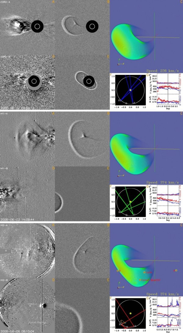
Figure 6. Three multipanel figures comparing real and synthetic images, representative of COR2, HI1, and HI2 data. Each frame consists of a STEREO-A image (A), a STEREO-B image (D), our evolving 3D model CME (C), and synthetic images computed from this model ((B) and (E)). Panel (C) has a CME speed indicator in its lower right corner. In the HI2 frame, panel (C) also shows the locations of STEREO-A, STEREO-B, Earth, and Comet Boattini. Panel (F) shows the locations of the model CME, STEREO-A, STEREO-B, and Earth (⊕) in the ecliptic plane, along with colored lines indicating the fields of view of the instruments used in panels (A) and (D). Panel (G) shows in situ measurements of proton density, velocity, and magnetic field from STEREO-A and STEREO-B.(An animation of this figure is available in the onldine journal.)
Download figure:
Standard image High-resolution imageThe COR2 frame of Figure 6 illustrates how the CME's appearance at early times can be reproduced by a flux rope with a significant 35° tilt relative to the ecliptic, as long as it is a fat flux rope. The two subsequent HI1 and HI2 frames illustrate how narrowing and flattening the flux rope can explain the evolving shape of the CME in the STEREO-A images, although only the central part of the CME is really visible in the HI2-A image. This demonstrates that it is possible to reproduce the changing appearance of the CME without requiring any rotation of the structure between the COR2-A and HI1-A fields of view. The HI2 frame also shows the location of the 3D flux rope relative to Earth, the two STEREO spacecraft, and Comet Boattini at a time shortly before the CME strikes STEREO-B and the comet.
Although the model reproduces the shape of the outer edge of the CME flux rope reasonably well, the HI1 panel of Figure 6 shows that the model is not as successful in fitting the shape and latitudinal extent of the inner edge. The outline of the flux rope inner edge suggested by the model is much too pointed. This is an indication of the limitations of our parameterized flux rope shape, as no combination of parameters will rectify this problem. To be specific, Equation (4) simply will not yield an inner edge shape that will better reproduce the observations. A more precise replication would probably require a functional form that allows the legs of the loop to start very close together and then expand away from each other super-radially, something Equation (4) does not allow.
The STEREO mission promises to greatly improve our understanding of the angular extent of CMEs in the inner heliosphere. An angular extent for our model CME in the plane of the flux rope can be estimated by first setting r(
The in situ data panel in the HI2 frame shows the two density peaks seen by STEREO-B when the CME hits, which are discussed in much more detail by Möstl et al. (2009). The two peaks correspond nicely to the two parallel fronts observed in the HI2-A image, representing the front and back side of the flux rope. In movies, two broad but faint fronts are also observed to pass through the HI2-B field of view corresponding to these two density peaks, at the time when STEREO-B is being hit by the CME (see the HI2-B panel of Figure 1). This illustrates the HI2 telescope's unprecedented ability to image a flux rope CME from the inside. The synthetic images from the model are at least crudely able to match the appearance and timing of the HI2-B fronts, the first of which is most evident in its effect on Comet Boattini.
According to the model, the comet is struck by the west leg of the flux rope, while STEREO-B is struck by the central part, with the apex of the flux rope passing a little to the south of the spacecraft. Our model CME first hits STEREO-B at about 22:10 UT on June 6, within an hour of the CME front's arrival based on the in situ data. The timing of the CME's passage over the comet is not quite as successfully reproduced, with the model CME hitting the comet about 4 hr after the observed tail disconnection event. Nevertheless, requiring that our flux rope model strikes the comet at roughly the appropriate time represents a useful constraint on the model. Images at early times imply a flux rope tilt of ϕfr ≈ −45°, but in our best fit we reduce the tilt to ϕfr = −35° to keep the CME's west leg from being too much to the south to hit the comet squarely.
Möstl et al. (2009) estimate a flux rope tilt of about ϕfr = −45° based on an analysis of STEREO-B's in situ measurements of the event. Our assessment solely from the images is nicely consistent with their measurements. It is very encouraging that two very different methods of analyzing CME flux rope orientation should yield compatible results.
Most of the morphological evolution of this CME seems to occur in the HI1 field of view. It is probably not a coincidence that this is also where the CME reaches its terminal velocity of about 400 km s−1. The morphological changes are presumably driven mostly by the CME's interactions with the ambient solar wind, but perhaps internal forces within the CME's magnetic structure could also play a role. Reconstructions of CME evolution like that performed here could potentially provide modelers with valuable information in their efforts to understand how CMEs expand into the IPM and interact with their environment.
In Section 3, we discussed at length how different assumptions about the shape of the leading edge of the CME can lead to very different inferences about its kinematic behavior. The detailed morphological reconstruction of the CME in this section should in principle allow an even more precise connection to be established between measured elongation angle, , and inferred Sun-center distance, r. In other words, with the results of the morphological analysis in hand, we should be able to do better than the "harmonic mean" approximation that we decided in Section 3 was the best assumption for this particular CME.
Using experiments such as that in Figure 4 (but this time using the real leading edge shape from our morphological analysis), we can establish exactly what part of the CME front is being perceived as the leading edge as a function of time, and we can therefore connect the apparent leading edge distance to the actual distance of the central part of the CME front. Figure 7 shows that correcting our leading edge distances in this fashion leads to a kinematic behavior far from the Sun that is certainly more plausible than the simple fixed-ϕ and point-P approaches, and is similar to the preferred harmonic mean results (see Figure 2). However, despite the sophistication of this approach to the kinematic analysis, these new distance-versus-time measurements are not clearly superior to those from the harmonic mean approximation. In fact, a more detailed kinematic analysis to the new distance measurements in Figure 7 (analogous to that in Figure 5) yields a velocity and arrival time prediction at STEREO-B that are in slightly worse agreement with the STEREO-B in situ observations than the predictions from the harmonic mean approximation.
Figure 7. Distance and velocity measurements for the 2008 June 1 CME computed under the "fixed-ϕ" approximation assuming a trajectory of ϕ = 63°, as in Figure 2, and also after modifying the distances based on CME front shapes suggested by our best 3D morphological model. The modified velocities lack the implausible velocity increase seen in the unmodified measurements.
Download figure:
Standard image High-resolution image
We conclude that the complicated morphological corrections to CME kinematics represented in Figure 7 may not yield better results than the simpler approximations shown in Figure 2, and therefore will not generally be worth the effort. The morphological corrections carry their own questionable assumptions, despite the sophistication of the approach. In particular, the analysis implicitly assumes that the entire CME leading edge is visible at all times. In reality, the HI2-A images of the CME tell us that the most foreground parts of the CME fade as the CME moves through the HI2-A field of view, in contrast to the synthetic images. Presumably, there is simply not enough mass there for those parts of the CME front to be visible as the CME moves farther from the Sun. This introduces errors in our inferences about what part of the CME front is being seen as the leading edge as a function of time. And we believe these errors are primarily responsible for the morphological analysis not leading to better kinematics compared to the harmonic mean approximation.
5. SUMMARY
We have analyzed STEREO observations of the changing morphology of the 2008 June 1 CME and come to the following conclusions.
- 1.After expanding at a constant slow velocity of about 35 km s−1 through the COR1-A field of view, the leading edge of the CME accelerates through COR2-A to a terminal velocity of about 384 km s−1 28 R☉ from Sun-center in the HI1-A field of view.
- 2.The observed change in morphology is best explained by a flux rope rotated −35° from the ecliptic that flattens and narrows with time, with the greatest changes taking place at about the time the CME reaches its terminal velocity. No change in flux rope orientation is required to explain the data, only a change in its shape. The CME has an angular extent of about 70° in the plane of the flux rope.
- 3.Our inferred flux rope orientation agrees well with that inferred by Möstl et al. (2009) based solely on in situ observations of the CME from STEREO-B.
- 4.We infer a CME trajectory of ϕ = 63° from STEREO-A's location, consistent with previously published assessments.
- 5.The morphology and kinematics of our reconstructed CME reproduce the timing of the CME's observed interaction with Comet Boattini to within 4 hr, and the timing of its arrival at STEREO-B to within an hour.
- 6.Using the fixed-ϕ approximation to infer the kinematics of this CME leads to the inference of an implausible acceleration far from the Sun. In contrast, the harmonic mean approximation proposed by Lugaz et al. (2009) leads to more plausible kinematics and successfully reproduces the CME's velocity and arrival time observed by STEREO-B at 1
AU . - 7.Although the fixed-ϕ approximation does not work well for this event, it has worked well for other events that we have analyzed. The implication is that there is no single best method for getting from measured elongation angles to inferred CME Sun-center distances. Many methods should be tried for each event, with the method that leads to a constant velocity far from the Sun presumably being the best approximation.
The STEREO/SECCHI data are produced by a consortium of NRL (USA), LMSAL (USA), NASA/GSFC (USA), RAL (UK), UBHAM (UK), MPS (Germany), CSL (Belgium), IOTA (France), and IAS (France). In addition to funding by NASA, NRL also received support from the USAF Space Test Program and ONR. In addition to SECCHI, this work has made use of data provided by the STEREO PLASTIC and IMPACT teams, supported by NASA contracts NAS5-00132 and NAS5-00133.