


Abstract
Knots are fascinating topological structures that have been observed in various contexts, ranging from micro-worlds to macro-systems, and are conjectured to play a fundamental role in their respective fields. In order to characterize their physical properties, some topological invariants have been introduced, such as unknotting number, bridge number, Jones polynomial and so on. While these invariants have been proven to theoretically describe the topological properties of knots, they have remained unexplored experimentally because of the difficulty associated with control. Herein, we report the creation of isolated electrical knots based on discrete distributions of impedances in electric circuits and observation of the unknotting number for the first time. Furthermore, DNA structure transitions under the action of enzymes were studied experimentally using electrical circuits, and the topological equivalence of DNA double strands was demonstrated. As the first experiment on the creation of electrical knots in real space, our work opens up the exciting possibility of exploring topological properties of DNA and some molecular strands using electric circuits.
Export citation and abstract BibTeX RIS

Original content from this work may be used under the terms of the Creative Commons Attribution 4.0 licence. Any further distribution of this work must maintain attribution to the author(s) and the title of the work, journal citation and DOI.
1. Introduction
The exploration of knot physics has become one of the most fascinating frontiers in recent years, due to its complex topology that plays an important role in physical and life sciences [1–5]. At present, various knots have been constructed based on different physical implementations. According to the characteristics of the matter that forms the structure, the knots can be divided into two types. One is called a 'continuous' knot, which is formed by continuously distributed substances, such as knots in liquid crystal [6, 7], fluid [8–12], elastic media [13], momentum space [14], and light and acoustic systems [15–23]. The other is called the 'discrete' knot, which is formed by discrete lattices, such as knots in DNA and other molecular strands [24–32].
'Discrete' knots are usually found in the microscopic world, particularly on the cellular level. Different molecular knots can be synthesized through the accurate control of chemical reactions [1, 33–38]. After acting on duplex cyclic DNA molecules with direct repeats, enzymes called topoisomerases are able to generate different nontrivial DNA knots. Topoisomerases have shown to be tendentious in knotting or unknotting DNA molecules, which have completely different functions in living systems. For instance, type II topoisomerase manifests a preference to unknot DNA molecules. Therefore, understanding the possible topologies of DNA molecules is helpful to explore life mechanisms. In recent years, many theoretical investigations, including lattice-based simulations, equilateral chain model simulations, grid diagrams and so on, have proven to generate the topology of different DNA knots [35–38]. However, the direct experimental evidence of DNA topology, especially the topological equivalences between two different DNA structures, is still lacking.
In this work, we experimentally constructed the 'discrete' knots based on circuits [39–48], which differ from other realizations of 'continuous' knots for macroscopic objects. The advantage of constructing such an experimental platform is that it can be used to study various phenomena corresponding to DNA topology. For example, through the change of impendence in the electric circuits, we could for the first time have been able to render one important topological invariant in knot theory experimentally observable: namely, the unknotting number. The topological change of DNA molecules under the action of enzyme Tn3 resolvase was also observed. In addition, the topological equivalence between two different structures of DNA molecules was experimentally demonstrated using the circuit platforms.
2. Electrical realization of knots and observation of unknotting number
To implement electric knots in an electric circuit, the following steps were performed. At first, we established a connection between the knot theory and the corresponding construction in the lattice. The coupling strengths between sites in the lattice were designed, and the sites in the lattice occupied by the localized eigenstates comprised the knot structure. Then, we designed the electric circuit and correlated the Laplacian describing the circuit to the Hamiltonian in the lattice by choosing the appropriate electric capacitors and grounding elements. Finally, the distributions of impedance in the circuit were measured, where nodes possessing large impedances correspond to the sites occupied by localized eigenstates in the lattice and form the knot. The detailed construction method is described in appendix

Figure 1. Electric realizations of knots. (a) The construction of the trefoil knot in the electric circuit. The red cylinders represent the small electric capacitors C1 = 100 pF, and the blue cylinders denote the large electric capacitors C2 = 10 nF. Large red spheres indicate that the nodes possessing the impedance larger than 1 k
Download figure:
Standard image High-resolution imageIn order to observe such a phenomenon experimentally, we designed the corresponding circuits (the circuit corresponding to figure 1(a) is shown in figure 1(c)). For the convenience of experiment, the total cube was cut into three layers, which were then positioned on three printed circuit boards (PCBs). Capacitors were connected to every node on adjacent layers. A cyclic boundary condition was applied to avoid the edge effect. The experimental setup of the fabricated circuit is shown in figure 1(d). In one PCB layer, the capacitors are arranged on the front and grounding inductors on the back. The enlarged image of the front and back of a plaquette is given in figure 1(e). The fabricated sample has exactly the same construction as that shown in figure 1(a). The measurement results of impedances corresponding to the cases in figures 1(a) and (b) are presented in figure 1(f) and (g), respectively. Experimental details are given in appendix
Because circuit networks possess remarkable advantages of being tunable and reconfigurable, many interesting problems associated with the knot theory using electric knots can be explored. In mathematics, some invariants are usually introduced to describe the topological properties of knots, such as unknotting number, bridge number, Jones polynomial, and Alexander polynomial [1, 4, 5]. Although these concepts and theories have existed for around 100 years, they have never been proven by experiments. For the first time, this work provides the observation of these topological invariants in the designed circuit platforms. Particularly, one invariant, the unknotting number, is defined as the least times in the change of crossing to make the knot become an unknot. Thus, the key to observe the unknotting number is to realize the change of crossing in the electric circuit.
Figures 2(a)–(e) illustrate the change of one crossing in geometry, whereby such type of evolution process can be shown in the designed circuits. Figures 2(f)–(j) present the corresponding circuits, and construction details are provided in appendix
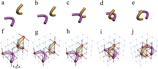
Figure 2. The change of one crossing in geometry and electric realizations. (a)–(e) We provide the process to change the crossing between the purple and the orange tube once. (f)–(j) Circuit designs to illustrate such changing process. In each panel, red (blue) cylinders between every two nodes represent the electric capacitors C1 = 100 pF (C2 = 10 nF). Red spheres denote the nodes with large impedances. We use purple and orange tubes to connect these nodes with large impedances.
Download figure:
Standard image High-resolution imageWe further studied the change of crossing in the knot structures, considering the transition from the electrical trefoil knot in figure 1(a) to unknot in figure 1(b). In the transition process, the change of crossing occurs only once, which was observed in the designed circuit by continuously modulating the capacitors and associated grounding elements. The detailed discussions and experimental results are presented in appendix
Similarly, other invariants such as the bridge number, Jones polynomial and Alexander polynomial, can also be observed experimentally by designing the corresponding circuits. An important feature of electric knots is their discrete distributions of impedances, which enables us to study the topological properties of molecular strands. For example, the phase transition of DNA structures and topological equivalence problems of DNA double strands can be discussed by designing circuit platforms.
3. Observation of the topological phase transition in DNA structures using electrical circuits
It is known that the duplex cyclic DNA molecule can show the structures of knots and links under the action of topoisomerases. In living systems, knotting and unknotting DNA molecules have totally different functions, whereby different knots and links of DNA molecules can appear when enzyme Tn3 resolvase is applied with direct repeats [1, 2, 33, 34]. Before the action of Tn3 resolvase, the DNA molecule can be viewed as two tangle structures, as shown in figure 3(a), where one substrate tangle S is not affected by Tn3 resolvase and the other site tangle T is influenced by Tn3 resolvase. In this case, the DNA molecule is unknotted. After one action of Tn3 resolvase, the site tangle T is replaced by the recombination tangle R, and the geometric structure of DNA molecule changes to that of a one hopf link, as shown in figure 3(d).
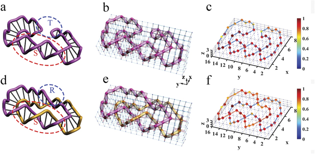
Figure 3. Electrical realizations of different DNA molecular structures before and after the action of topoisomerase. (a) and (d) The structures of DNA before and after the action of the enzyme Tn3 resolvase. In (a), the structure of DNA is composed by one substrate tangle S and the other site tangle T. In (d), after the action of Tn3 resolvase, the site tangle T is replaced by the recombination tangle R. (b) and (e) The electric realizations of different DNA structures before and after the action of Tn3 resolvase. In each panel, red (blue) cylinders between every two nodes represent the electric capacitors C1 = 100 pF (C2 = 10 nF). Red spheres denote the nodes with large impedances. We connect these nodes in purple and orange tubes. (c) and (f) The distributions of impedances in experimentally electric circuits. All the values of impedance are normalized to the largest impedance in each panel. We use the solid lines to connect the nodes with large impedance.
Download figure:
Standard image High-resolution imageThe corresponding circuits can be constructed to display the above phenomenon very well. Figures 3(b) and (e) display the designed circuits corresponding to the structures in figures 3(a) and (d), respectively. In the circuits, different electric capacitors are chosen to connect the two nearest neighboring nodes. In the figure, the structural functions of DNA molecules are integrated into the design of circuits, where red spheres denote the nodes with impedances larger than 1 k
The above discussions present only one phase transition of DNA molecules from the unknotted structure to the hopf link under the action of topoisomerases. In fact, multiple phase transitions can occur when the topoisomerases react repeatedly. For example, the structure of DNA molecules in figure 3(d) transitioned into the figure-8 knot structure when enzyme Tn3 resolvase was continuously applied. Such multiple phase transitions can also be well demonstrated in designing circuits by modulating the capacitors and associated grounding elements (see appendix
4. Demonstration of topological equivalence of DNA double strands in the electric circuit
DNA double strands play a dominant role in various biological functions that are necessary for life, such as replication, transcription and recombination [1, 2]. Cyclic duplex DNA exhibits different geometric structures under different ambient environments. Figure 4(a) shows the cyclic duplex DNA structure in the relaxed state, which becomes an intermediate state (figure 1(d)) with the change of ambient environment, and then transitions into an unrelaxed state (figure 4(g)). In the unrelaxed state, the DNA structure is more tightly twisted. To describe the different geometric structures of cyclic duplex DNA, the twist (Tw) is defined as how much the DNA structure twists around its axis, and the writhe (Wr) refers to how much the axis of the DNA structure is contorted in space [1, 49, 50]. When the cyclic duplex DNA structure is in the relaxed state (figure 4(a)), it does not twist around its axis; instead, its axis is contorted once in space and, thus, the Tw = 0 and Wr = 1. In figure 4(g), the axis of the DNA structure lies flat in the plane, but the structure twists around its axis once, and thereby, Tw = 1 and Wr = 0.
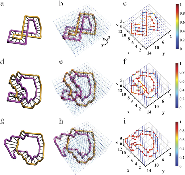
Figure 4. Electric demonstration of topological equivalence between different DNA structures. (a) The simplest DNA structure with the twist Tw = 0 and the writhe Wr = 1. (b) The electric design of (a). (c) The experimental distribution of impedance in the electric circuit for (b). (d) The DNA structure in the middle of the change process. (e) The electric design of (d). (f) The experimental distribution of impedance for (e). (g) The DNA structure with the twist Tw = 1 and the writhe Wr = 0. (h) The electric design of (g). (i) The experimental distribution of impedance for (h). In panel (b), (e) and (h), red (blue) cylinders between every two nodes represent the electric capacitors C1 = 100 pF (C2 = 10 nF). Red spheres denote the nodes with large impedances. In panel (c), (f) and (i), all the values of impedances are normalized to the largest one, and we use the solid lines to connect the nodes with large impedances.
Download figure:
Standard image High-resolution imageThe topology of the DNA geometric configuration determines the functions of living mechanisms. The linking number Lk = Tw + Wr is usually introduced to characterize the topological properties of different geometric configurations. It has been proven that, although the geometric configuration is different, the linking number is the same, and the function of DNA is the same. This is called the topological equivalence. For example, the two geometric configurations shown in figures 4(a) and (g) seem different, yet their linking numbers are the same.
The demonstration of topological equivalence between two different geometric configurations is very meaningful, but is very difficult to experimentally demonstrate in living cells. Using the designed circuit platforms, we were able to observe the phenomena very well. By integrating the cyclic duplex DNA structure function in the relaxed state into the circuit design, we constructed a circuit that displays the DNA configuration (figure 4(b)). Similar to the above figures, red spheres denote the nodes with impedances larger than 1 k
By tuning the capacitors and associated grounding elements, the corresponding circuits for the intermediate state (figure 4(d)) and unrelaxed state (figure 4(g)) were also obtained, which are shown in figures 4(e) and (h), respectively. The fabricated details and measured process for these designed circuits are described in appendix
Therefore, to demonstrate the topological equivalence between the structures, a continuous change from one structure to another needed to occur. That is, there is no change of crossing in the process. In fact, in the designed circuits, it is convenient to study the continuous change between two structures by modulating the electric capacitors and related grounding inductors step-by-step. Details of the change process for such a case are given in appendix
5. Conclusion
This work theoretically and experimentally proposes schemes to create isolated electrical knots based on discrete distributions of impedances in electric circuits. Using the designed circuit platforms, we experimentally observed unknotting numbers for the first time, and the corresponding DNA structure transitions under the action of enzymes using electrical circuits. The topological equivalence of DNA double strands was further demonstrated experimentally. Our results provide convincing evidence that the electric circuits offer reliable platforms to study the various topological properties of knots and links, especially microscopic 'discrete' knots in the molecular strands. Moreover, such circuit platforms revealed new phenomena in this work and also provide a basis for future exploration of unsolvable problems.
Acknowledgments
This work was supported by the National key R & D Program of China under Grant No. 2017YFA0303800 and the National Natural Science Foundation of China (Nos. 91850205 and 61421001).
Data availability statement
All data that support the findings of this study are included within the article (and any supplementary files).
Appendix A.: The general scheme to create electrical knots
Here, we describe how to construct knots and links in electric circuits. We start from the standard procedure of obtaining the knots and links, and then provide the design on the circuit.
A.1. Construction of standard knots
According to the theory [1, 2], since the abstract group definitions of braids have remarkable geometric and topological interpretation, the knots and links can be obtained from the braids. The braided function is expressed with a formal variable u and has N distinct zeros at positions parameterized by the height h in equation (A1) as

Since the knots or links are composed by closed braids, the braid function needs to be periodic in h. It is convenient that the range of h is taken from 0 to 2
The formal variables in the expression above can be mapped to the R3 space through the Milnor map. We use Cartesian coordinates x, y, and z to express the formal variables u and v in the following equations:
Given in both Cartesian and cylindrical coordinates, R2 = x2 + y2 and R eiϕ = x + iy, the expression for the standard trefoil knot is written as

In figure 5(a), we provide the standard trefoil knot in the R3 space.
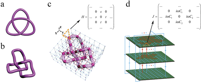
Figure 5. Details of electrical construction of trefoil knot in the circuit. (a) The standard trefoil knot. (b) The deformation of standard trefoil knot. (c) Construction of the trefoil knot (b) in the lattices. Red (blue) cylinders represent the couplings strengths t = 0.01 (s = 1). The Hamiltonian for three sites in the lattice is presented. (d) Realization of the trefoil knot (b) in the electric circuit. The value for capacitors in red (blue) is C1 = 100 pF (C2 = 10 nF). The Laplacian for three nodes in the circuit is presented explicitly.
Download figure:
Standard image High-resolution imageThe mathematic theory tells us that the knots and links can be deformed freely in space, but not allowed to be cut off or glued. After such a deformation process, the geometric structure representing the knot (link) can be changed to another structure. Although these two structures seem different at the first sight, they are actually the same knots (links). It is often called these two knots (links) are isotopic. It is hard to find an ambient isotopy function in general, the researchers often project the knot into two-dimension and manipulate this projection in three formal ways, i.e., the Reidemeister moves. These manipulations are equivalent to an ambient isotopy in 3D. In figure 5(b), we provide one structure obtained from the deformation of the structure in figure 5(a). These two are isotopic since they can be deformed into each other without being cut off or glued. The expression for the deformed trefoil knot in figure 5(b) is shown as
The deformed trefoil knot can be composed of two fitting curves when we set  . The ranges of coordinates are, x ∈ [2, 7] and y ∈ [2, 8], z ∈ [1, 2]. The values from a1 to a52 for these two fitting curves are listed below (table 1).
Table 1. The coefficients a1 to a52 in the fdeformed-tre. The values outside and inside [*] are the coefficients of the first and second fitting curves, respectively.
| a1 = 0.2353 − 0.0260i [−0.0332 + 0.0187i] | a2 = 0.0428 + 0.0102i [0.2930 + 0.0014i] |
| a3 = 1.2146 − 0.0230i [0.5328 + 0.0342i] | a4 = 0.0120 + 0.0014i [0.0226 + 0.0030i] |
| a5 = −0.0080 + 0.0050i [−0.0091 + 0.0021i] | a6 = −0.2362 + 0.0198i [−0.0899 − 0.0134i] |
| a7 = −0.0031 + 0.0032i [0.0015 − 0.0065i] | a8 = −0.0918 − 0.0084i [−0.0629 + 0.0063i] |
| a9 = −0.0973 + 0.0038i [0.1002 − 0.0328i] | a10 = (4.14 − 6.47i) × 10−4 [(1.39 + 2.17i) × 10−4] |
| a11 = −0.0008 − 0.0011i [0.0001 − 0.0012i] | a12 = −0.0133 − 0.0018i [0.0033 − 0.0012i] |
| a13 = (6.07 + 6.39i) × 10−4 [−0.0014 + 0.0007i] | a14 = −0.0009 + 0.0017i [−0.0061 + 0.0021i] |
| a15 = −0.0008 − 0.0053i [−0.0077 − 0.0027i] | a16 = −0.0002 + 0.0011i [−0.0025 + 0.0007i] |
| a17 = 0.0067 − 0.0053i [−0.0102 − 0.0009i] | a18 = 0.0063 + 0.0090i [−0.0179 + 0.0002i] |
| a19 = −0.0961 − 0.0017i [0.0048 + 0.0009i] | a20 = (−5.03 + 2.24i) × 10−4 [2.40 × 10⁻⁵ − 2.21 × 10⁻⁴i] |
| a21 = 1.99 × 10⁻⁷ + 9.17 × 10⁻¹¹i [2.04 × 10⁻⁴ − 6.26 × 10⁻⁵i] | a22 = (−2.00 + 3.23i) × 10−4 [2.82 × 10⁻⁵ − 1.02 × 10⁻⁴i] |
| a23 = (−1.49 − 2.91i) × 10−4 [(4.98 − 2.15i) × 10−4] | a24 = (4.17 + 5.27i) × 10−4 [(5.68 − 1.36i) × 10−4] |
| a25 = 0.0075 − 0.0009i [0.0028 + 0.0004i] | a26 = 1.43 × 10⁻⁸ − 1.34 × 10⁻¹⁰i [−2.04 × 10⁻⁴ + 6.26 × 10⁻⁵i] |
| a27 = (−3.04 − 3.20i) × 10−4 [(8.81 − 3.23i) × 10−4] | a28 = 0.0024 + 0.0014i [0.0027 + 0.0010i] |
| a29 = 0.0301 − 0.0025i [(−9.02 − 9.53i) × 10−4] | a30 = 4.80 × 10⁻⁵ − 1.67 × 10⁻⁴i [(−7.31 − 1.66i) × 10−5] |
| a31 = 8.69 × 10⁻⁵ − 5.31 × 10⁻⁴i [0.0018 − 0.0001i] | a32 = 0.0002 + 0.0015i [−0.0008 + 0.0016i] |
| a33 = 0.0144 − 0.0036i [−0.0053 − 0.0024i] | a34 = −0.0264 + 0.0001i [−0.0103 + 0.0040i] |
| a35 = −8.94 × 10⁻⁹ + 3.04 × 10⁻¹⁰i [2.17 × 10⁻⁶ − 6.61 × 10⁻⁷i] | a36 = −9.83 × 10⁻¹⁰ + 1.05 × 10⁻¹¹i [(−6.54 + 1.99i) × 10−6] |
| a37 = −7.47 × 10⁻¹¹ + 8.59 × 10⁻¹²i [(6.54 − 1.99i) × 10−6] | a38 = −1.69 × 10⁻⁹ + 7.38 × 10⁻¹¹i [−2.19 × 10⁻⁶ + 6.63 × 10⁻⁷i] |
| a39 = 6.85 × 10⁻⁴ − 2.23 × 10⁻⁵i [(−3.37 + 2.62i) × 10−4] | a40 = (2.47 + 2.40i) × 10−4 [(−4.29 + 4.22i) × 10−4] |
| a41 = −3.19 × 10⁻⁵ + 1.33 × 10⁻⁴i [8.76 × 10⁻⁵ − 3.78 × 10⁻⁶i] | a42 = −2.18 × 10⁻⁴ − 4.50 × 10⁻⁵i [(4.24 − 6.04i) × 10−5] |
| a43 = (−8.64 − 4.71i) × 10−5 [(1.38 − 1.34i) × 10−4] | a44 = 3.75 × 10⁻⁶ − 2.47 × 10⁻⁵i [(4.62 − 3.25i) × 10−5] |
| a45 = −0.0027 + 0.0006i [(5.32 − 1.65i) × 10−4] | a46 = −0.0014 + 0.0001i [5.51 × 10⁻⁵ + 4.07 × 10⁻⁴i] |
| a47 = 3.65 × 10⁻⁴ + 6.14 × 10⁻⁵i [−9.15 × 10⁻⁵ + 1.23 × 10⁻⁴i] | a48 = −7.50 × 10⁻⁶ + 4.94 × 10⁻⁵i [(−9.12 + 9.36i) × 10−5] |
| a49 = 0.0056 + 0.0002i [0.0014 − 0.0006i] | a50 = −4.65 × 10⁻⁴ − 6.80 × 10⁻⁵i [−1.32 × 10⁻⁴ − 1.03 × 10⁻⁵i] |
| a51 = 2.49 × 10⁻⁷ − 7.61 × 10⁻⁹i [1.41 × 10⁻⁷ − 2.71 × 10⁻⁸i] | a52 = 6.17 × 10⁻⁸ − 2.37 × 10⁻⁹i [1.83 × 10⁻⁷ − 2.67 × 10⁻⁸i] |
A.2. Mapping process
The previous step has shown how to obtain one knot or link in space. Figures 5(a) and (b) show the trefoil knot. Here we provide the construction of trefoil knot in the lattice. We construct the lattice as

The site in the lattice is often described by the integral coordinate. In figure 5(c), the ranges of x, y, z coordinates in the lattice are x ∈ [1, 7], y ∈ [1, 8], z ∈ [0, 2], and the values of x, y, z are all integers. Therefore, we seek all integral coordinates satisfying  and the sites described by these coordinates can comprise the deformed 'discrete' trefoil knot. We list all these coordinates in sequence below.
In the Hamiltonian, we set the coordinates shown in table 2 to connect with the six adjacent sites through the coupling strength ti,j = 0.01, and the coupling strengths between other sites are sk,l = 1. We provide the construction of this Hamiltonian in the three-dimensional lattice in figure 5(c). Red (blue) cylinders represent the coupling strength ti,j (sk,l ). We also show the distribution of localized eigenstates of H in figure 5(c). Red spheres label the sites occupied by the localized eigenstates. We find that the coordinates of these sites are exactly those shown in table 2. To illustrate the distribution clearly, we use the purple tube in figure 5(c) to connect these sites and find that they comprise the trefoil knot. This trefoil knot is the 'discrete' deformed trefoil knot in figure 5(b).
Table 2. The coordinates  satisfy
  .
.
| (2,3,2) | (2,4,1) | (3,5,1) | (4,6,1) | (5,6,2) | (6,5,2) | (7,4,2) | (6,3,2) | (5,3,1) |
| (4,4,1) | (4,5,2) | (3,6,2) | (4,7,2) | (5,8,2) | (6,7,2) | (6,6,1) | (5,5,1) | (5,4,2) |
| (4,3,2) | (3,2,2) |
A.3. Electric realization
Since the lattice contains three layers along the z direction, we use three PCB layers in the electric circuit. The detailed structure is provided in figure 5(d). Every two nearest neighboring nodes in the circuit is connected through the capacitor C1 (C2), which corresponds to the coupling strength ti,j (sk,l ) in the lattice. In the electric design, the dynamics of this circuit can be described by one Laplacian J which bridges the current and voltages in the circuit. By choosing appropriate grounding inductors, we can make the Laplacian J similar to the Hamiltonian Hdef-tre. For three nodes in the circuit (contained in the orange dotted triangle) in figure 5(d), the Laplacian is addressed as
In our design, when we set  , the diagonal elements in the matrix J are eliminated, and the Laplacian changes to the expression shown in the inset of figure 5(d).
In our experiment, we use the impedance as the measured quantity. The impedance between ath node and bth node is  . Here, Va
(Vb
) is the electric potential at a (b)th node and Ia,b
is the current between ath node and bth node. The symbols jn
and
. Here, Va
(Vb
) is the electric potential at a (b)th node and Ia,b
is the current between ath node and bth node. The symbols jn
and
After completing these three steps, we realize the 'discrete' trefoil knot in the electric circuit. To make this realization clear, we connect these 'special' nodes having large impedances together. Since these nodes distribute at the diagonal nodes of each plaquette in the circuit (red spheres in figure 1(a) and large spheres in figure 1(f) of the main text), we connect these diagonal nodes of each plaquette in the circuit in sequence. The obtained connection is exactly the trefoil knot (see figure 1(a) and (f) in the main text). Compared with other experimental realizations of knots, the realization of trefoil knot in the electric circuit is easy and controllable. Moreover, not only the trefoil knot is implemented electrically, other knots and links can also be realized in the electric circuit in the same way.
Appendix B.: The experimental details in the electric circuit
Here, we describe the experimental details in the electric circuit. In our experiment, we choose the electric capacitors CC41-0603-CG-50V-100pF-F(N) and CC41-0603-CG-50V-10nF-F(N), which are described as the small capacitors in red (C1) and the large capacitors in blue (C2) in the main text, respectively. The types of inductors are NLV32T-3R3J-EF and NLV32T-033J-EF. We measure the impedance at each node by connecting the impedance analyzer to the measurement connectors. The cooper pillars are connected to the grounding inductors, which also sustain the three PCB layers.
We use the WK6500B impedance analyzer to measure the impedance. In principle, we need to measure the impedance between the nodes and the ground at the resonant frequency  . Due to the existence of various errors in the experiments, the measured frequency is a little smaller than the resonant frequency. To obtain the appropriate results, we use the impedance analyzer to sweep the frequencies around the resonant frequency. We choose the certain frequency where the peak of impedance appears and we use this peak value as the impedance of this node.
In our experiment, the values of electric inductors and capacitors, of course, are not ideal, and there exists spurious inductive coupling in the experimental setup, but the dominant error is from the connecting wires. The type of these wires is DB9. These wires are used to realize cyclic boundary condition and connect different PCB layers. The parasitic inductance from long connecting wires cannot be neglected. When we measure the impedance of nodes connecting with adjacent nodes through the small electric capacitor C1, the impedance of these nodes are very large in the ideal circuit simulation. However, in fact, due to the non-negligible parasitic inductance of the long wires in the experiment, we find that the impedances for these nodes at the edge of the PCB layer are often a little bit smaller than those at the inner part of the layer, but are still much larger than the nodes with small impedances. So this error does not ruin our experimental results.
Appendix C.: The realization of change process in the lattice and electric circuit
Here, we describe how to realize the change process in the electric circuit. Similar to the construction in appendix A, we firstly provide the functions describing the curves from figures 2(a)–(e) of the main text, then we give the Hamiltonians of lattices corresponding to the electric designs from figures 2(f)–(j) of the main text.
The functions from figures 2(a)–(e) in the main text are listed below in sequence:


Here we provide the constructions of these five structures in the lattices. The ranges of x, y, z coordinates in the lattices are x ∈ [1, 4], y ∈ [1, 3], z ∈ [1, 4], and the values of x, y, z are all integers. We construct the lattices as

The sites in the lattices are often described by the integral coordinates. Therefore, we seek all integral coordinates satisfying  and
and  . We list all these coordinates in sequence below.
In the Hamiltonian, we set the coordinates shown in table 3 to connect with the six adjacent sites through the coupling strength ti,j = 0.01, and the coupling strengths between other sites are sk,l = 1. We provide the construction of these Hamiltonians in these three-dimensional lattices from figures 6(a)–(e). Red (blue) cylinders represent the coupling strength ti,j (sk,l ). We also show the distribution of localized eigenstates of H from figures 6(a)–(e).
Table 3. The coordinates  satisfy
  and
and  .
.

|

| |
|---|---|---|
| i = a | (1,1,2), (2,2,2), (1,3,2) | (4,2,2), (3,2,3), (4,2,4) |
| i = b | (1,1,2), (2,2,2), (1,3,2) | (4,2,1), (3,2,2), (4,2,3) |
| i = c | (1,1,2), (2,2,2), (1,3,2) | (3,2,1), (2,2,2), (3,2,3) |
| i = d | (2,1,2), (3,2,2), (2,3,2) | (3,2,1), (2,2,2), (3,2,3) |
| i = e | (3,1,2), (4,2,2), (3,3,2) | (3,2,1), (2,2,2), (3,2,3) |
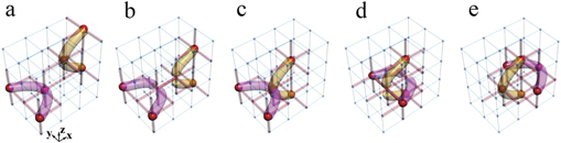
Figure 6. Constructions of the geometric structures shown from figures 2(a)–(e) in the main text. Red (blue) cylinders represent the couplings strengths t = 0.01 (s = 1). Red spheres in the lattices are the sites occupied by the localized eigenstates.
Download figure:
Standard image High-resolution imageRed spheres label the sites occupied by the localized eigenstates. We find that for the cases i = a, c, e, the coordinates of these sites are exactly those shown in table 3. But for the case i = b, the sites with coordinates (2,2,2) in  and (3,2,2) in
  are not occupied by the localized eigenstates; and for the case i = d, the sites with coordinates (3,2,2) in
  and (2,2,2) in
  are not occupied by the localized eigenstates. So if we connect the sites occupied by the localized eigenstates, we can obtain the corresponding geometric structures depicted in figures 2(a), (c) and (e) in the main text, but not obtain the corresponding geometric structures depicted in figures 2(b) and (d) in the main text. This is because, in the lattice, when the sites connect with neighboring sites by ti,j
or sk,l
, the hopping rate between sites shown in Hamiltonian is ti,j
or sk,l
. Consider ti,j
< sk,l
, so electrons are more likely trapped at the site connected to neighboring sites by ti,j
. But when two sites connecting with neighboring sites by ti,j
connect directly, electrons are not limited to be at one of these two sites, which does not bring strong localization at these two sites simultaneously. If we still connect the sites occupied by localized eigenstates, we can find the connections are broken apart in the middle, see figures 6(b) and (d). So we cannot recover the geometric structures in figures 2(b) and (d) of the main text, respectively. It means that during the change of one crossing between two tubes, the sites occupied by localized eigenstates cannot correspond to the geometric structures twice. It is noted that this phenomenon does not have any influence on counting the times of changing crossings in the lattice.
are not occupied by the localized eigenstates. So if we connect the sites occupied by the localized eigenstates, we can obtain the corresponding geometric structures depicted in figures 2(a), (c) and (e) in the main text, but not obtain the corresponding geometric structures depicted in figures 2(b) and (d) in the main text. This is because, in the lattice, when the sites connect with neighboring sites by ti,j
or sk,l
, the hopping rate between sites shown in Hamiltonian is ti,j
or sk,l
. Consider ti,j
< sk,l
, so electrons are more likely trapped at the site connected to neighboring sites by ti,j
. But when two sites connecting with neighboring sites by ti,j
connect directly, electrons are not limited to be at one of these two sites, which does not bring strong localization at these two sites simultaneously. If we still connect the sites occupied by localized eigenstates, we can find the connections are broken apart in the middle, see figures 6(b) and (d). So we cannot recover the geometric structures in figures 2(b) and (d) of the main text, respectively. It means that during the change of one crossing between two tubes, the sites occupied by localized eigenstates cannot correspond to the geometric structures twice. It is noted that this phenomenon does not have any influence on counting the times of changing crossings in the lattice.
Consider the electric realizations correspond to the lattices, the distributions of impedance can exactly recover the geometric structures for cases i = a, c, e, but not form the structures for cases i = b, d. The electric simulation results of impedances for cases i = a, b, c, d, e are provided from figures 2(f)–(j) in the main text.
Appendix D.: The observation of unknotting numbers for trefoil knot, figure-8 knot and 83 knot in the electric circuits
D.1. Trefoil knot
When we change one crossing in the trefoil knot, the trefoil knot can change to the unknot. Here we provide the realizations of structures during the change process from figures 7(a)–(e).

Figure 7. Constructions to show the continuous change process from the trefoil knot to unknot. From (a)–(e), we illustrate the constructions from the trefoil knot to unknot in the lattices. Red (blue) cylinders represent the coupling strengths t = 0.01 (s = 1). Red spheres in the lattices are the sites occupied by the localized eigenstates. (f) Electric designs to realize the five lattices from (a)–(e). The gray regions are different for five structures from (a)–(e). Details in the gray region for (a)–(e) are provided in (f1)–(f5), respectively. The value of capacitors in red (blue) is C1 = 100 pF (C2 = 10 nF). (g) The experimental setup to realize these five structures.
Download figure:
Standard image High-resolution imageConstructions of these structures are similar to the description in appendix A. These five structures from figures 7(a)–(e) are constructed in the lattices as equation (D1),

The first structure is to form the trefoil knot and the fifth structure is to form the unknot. The construction for the first structure has been provided in appendix A. The functions for the four structures from figures 7(b)–(e) can be obtained in a similar way as the deformed trefoil knot (equation (A4)). Consider the lengthy expressions of these functions for these four structures, we do not provide the details of functions here. Since the coordinates in the lattice are integers, we provide the coordinates satisfying the corresponding functions in table 4. In our design, the coordinates in table 4 connect with the six adjacent sites through the coupling strength ti,j = 0.01, and the coupling strengths between other sites are sk,l = 1.
Table 4. The coordinates  connect with all adjacent sites through ti,j
= 0.01.
connect with all adjacent sites through ti,j
= 0.01.
| The second structure in figure 7(b) | ||||||||
| (2,3,2) | (2,4,1) | (3,5,1) | (4,6,1) | (5,6,2) | (6,5,2) | (7,4,2) | (6,3,2) | (5,3,1) |
| (4,4,1) | (4,5,1) | (3,6,2) | (4,7,2) | (5,8,2) | (6,7,2) | (6,6,1) | (5,5,1) | (5,4,2) |
| (4,3,2) | (3,2,2) | |||||||
| The third structure in figure 7(c) | ||||||||
| (2,3,2) | (2,4,1) | (3,5,1) | (4,6,1) | (5,6,2) | (6,5,2) | (7,4,2) | (6,3,2) | (5,3,1) |
| (4,4,1) | (3,5,1) | (3,6,2) | (4,7,2) | (5,8,2) | (6,7,2) | (6,6,1) | (5,5,1) | (5,4,2) |
| (4,3,2) | (3,2,2) | |||||||
| The fourth structure in figure 7(d) | ||||||||
| (2,3,2) | (2,4,1) | (3,4,1) | (4,5,1) | (5,6,2) | (6,5,2) | (7,4,2) | (6,3,2) | (5,3,1) |
| (4,4,1) | (3,5,1) | (3,6,2) | (4,7,2) | (5,8,2) | (6,7,2) | (6,6,1) | (5,5,1) | (5,4,2) |
| (4,3,2) | (3,2,2) | |||||||
| The fifth structure (the unknot in figure 1(b) of the main text) in figure 7(e) | ||||||||
| (2,3,2) | (2,4,1) | (3,4,2) | (4,5,2) | (5,6,2) | (6,5,2) | (7,4,2) | (6,3,2) | (5,3,1) |
| (4,4,1) | (3,5,1) | (3,6,2) | (4,7,2) | (5,8,2) | (6,7,2) | (6,6,1) | (5,5,1) | (5,4,2) |
| (4,3,2) | (3,2,2) |
Comparing the chosen coordinates in table 4 to realize the five structures in the lattices, we find that the coordinates from the first to the fifth structure are changed as: first (figure 7(a)) → second (figure 7(b)), (4,5,2) → (4,5,1); second (figure 7(b)) → third (figure 7(c)), (4,5,1) → (3,5,1); third (figure 7(c)) → fourth (figure 7(d)), (3,5,1) → (3,4,1), (4,6,1) → (4,5,1); and fourth (figure 7(d)) → fifth (figure 7(e)), (3,4,1) → (3,4,2), (4,5,1) → (4,5,2). In the change process, only one or two sites coupled to neighboring sites by strength ti,j = 0.01 are changed and these sites are nearest neighboring to each other at any two adjacent steps. In this sense, we can view this change process continuously. It means that we need only continuously to modulate some coupling strengths at each step in the change process. Red spheres from figures 7(a)–(e) are the occupations of localized eigenstates. We can find that for the first trefoil knot (figure 7(a)), the third structure (figure 7(c)) and the fifth unknot (figure 7(e)), the coordinates of sites occupied by the localized eigenstates are exactly those presented in tables 2 and 4; but for the second (figure 7(b)) and fourth (figure 7(d)) structures, some sites with coordinates shown in table 4 are not occupied by localized eigenstates. This phenomenon corresponds to the description of changing one crossing in the text around figure 6. Moreover, if we change the structures continuously following the sequence as, first (figure 7(a)), second (figure 7(b)), third (figure 7(c)), second (figure 7(b)) and first (figure 7(a)) structures, there are also two cases where the connections formed by localized eigenstates cannot recover the geometric structures. During this change, the trefoil return back to itself finally. Fortunately, the definition of unknotting number is the least time of crossing change necessary to change the knot into an unknot [1]. So the change making trefoil return back to itself is meaningless for the invariant unknotting number.
The corresponding electric realizations are presented in figure 7(f). Similar to the electric realization in appendix A, we connect every two nearest neighboring nodes in the electric circuit through the capacitors. The nodes with the coordinates presented in table 4 are connected by the small electric capacitor C1 = 100 pF. Other nodes are connected by the large capacitor C2 = 10 nF. Consider the correspondence between the lattice and the electric circuit, we need to change some capacitors and their associated grounding inductors at each step. The corresponding electric setup is presented in figure 7(g).
In figure 8, we provide the measurement outcomes of distributions of impedances for the corresponding electric designs in figure 7(f1)–(f5).
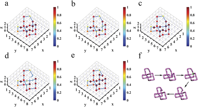
Figure 8. Experimental distributions of impedance for the five structures from trefoil knot to unknot. From (a)–(e), the value of impedance at each node has been normalized to the maximum value. (f) The structures recovered from the distributions of large impedances during the change in the circuit.
Download figure:
Standard image High-resolution imageFrom the distributions of impedance in figure 8, we can find that the nodes connected by small electric capacitors C1 are exactly having a large impedance for the first, third and fifth cases (figures 8(a), (c) and (e)). But for the second and fourth cases (figures 8(b) and (d)), some nodes connected by the capacitors C1 are not possessing large impedances. So these experimental results are consistent with those in the simulations.
D.2. Figure-8 knot
Not only the change of crossing once in the trefoil knot can be revealed in the electric circuit, but changes of crossings in other knots can also be provided. The construction details in the figure-8 knot and 83 knot are the same as the electrical trefoil knot above. We firstly provide the constructions of figure-8 knot and 83 knot in lattices, then map to the electric circuits. The Hamiltonian to realize the change from figure-8 knot to unknot in the lattice is shown as,

Here, we do not provide the details of functions for these structures from figure-8 knot to unknot. Consider the coordinates in the lattices are integers, we only provide the integral coordinates satisfying the corresponding functions in table 5. To realize the construction from the figure-8 knot to unknot, we show the coordinates in table 5 that connect with the six adjacent sites through the coupling strength ti,j = 0.01, and the coupling strengths between other sites are sk,l = 1.
Table 5. The coordinates  connect with all adjacent sites through ti,j
= 0.01.
connect with all adjacent sites through ti,j
= 0.01.
| The first structure (figure-8 knot) in figure 9(a) | ||||||||||
| (2,2,2) | (2,3,3) | (2,4,2) | (2,5,3) | (3,6,3) | (4,7,3) | (5,6,3) | (6,6,2) | (5,6,1) | (4,5,1) | (4,4,2) |
| (3,3,2) | (3,2,3) | (3,1,2) | (4,1,1) | (5,2,1) | (5,3,2) | (6,4,2) | (5,5,2) | (4,6,2) | (5,7,2) | (6,7,1) |
| (7,7,2) | (7,6,1) | (7,5,2) | (7,4,1) | (7,3,2) | (6,2,2) | (5,1,2) | (4,2,2) | (3,2,1) | ||
| The second structure in figure 9(b) | ||||||||||
| (2,2,2) | (2,3,3) | (2,4,2) | (2,5,3) | (3,6,3) | (4,7,3) | (5,6,3) | (6,6,2) | (5,6,1) | (4,5,1) | (4,4,2) |
| (3,3,2) | (3,2,3) | (3,1,2) | (4,1,1) | (5,2,1) | (5,3,2) | (6,4,2) | (5,5,2) | (4,6,2) | (5,7,2) | (6,7,1) |
| (7,7,2) | (7,6,1) | (7,5,2) | (7,4,1) | (7,3,2) | (6,2,2) | (5,1,2) | (4,2,2) | (3,2,2) | ||
| The third structure in figure 9(c) | ||||||||||
| (2,2,2) | (2,3,3) | (2,4,2) | (2,5,3) | (3,6,3) | (4,7,3) | (5,6,3) | (6,6,2) | (5,6,1) | (4,5,1) | (4,4,2) |
| (3,3,2) | (3,2,3) | (3,1,2) | (4,1,1) | (5,2,1) | (5,3,2) | (6,4,2) | (5,5,2) | (4,6,2) | (5,7,2) | (6,7,1) |
| (7,7,2) | (7,6,1) | (7,5,2) | (7,4,1) | (7,3,2) | (6,2,2) | (5,1,2) | (4,2,2) | (3,1,2) | ||
| The fourth structure in figure 9(d) | ||||||||||
| (2,2,2) | (2,3,3) | (2,4,2) | (2,5,3) | (3,6,3) | (4,7,3) | (5,6,3) | (6,6,2) | (5,6,1) | (4,5,1) | (4,4,2) |
| (3,3,2) | (3,2,2) | (3,1,2) | (4,1,1) | (5,2,1) | (5,3,2) | (6,4,2) | (5,5,2) | (4,6,2) | (5,7,2) | (6,7,1) |
| (7,7,2) | (7,6,1) | (7,5,2) | (7,4,1) | (7,3,2) | (6,2,2) | (5,1,2) | (4,2,2) | (3,1,2) | ||
| The fifth structure in figure 9(e) | ||||||||||
| (2,2,2) | (2,3,3) | (2,4,2) | (2,5,3) | (3,6,3) | (4,7,3) | (5,6,3) | (6,6,2) | (5,6,1) | (4,5,1) | (4,4,2) |
| (3,3,2) | (3,2,1) | (3,2,1) | (4,1,1) | (5,2,1) | (5,3,2) | (6,4,2) | (5,5,2) | (4,6,2) | (5,7,2) | (6,7,1) |
| (7,7,2) | (7,6,1) | (7,5,2) | (7,4,1) | (7,3,2) | (6,2,2) | (5,1,2) | (4,2,2) | (3,1,2) |
When compared with the chosen coordinates to realize the five structures in the lattices, in table 5, we find that the coordinates from the first to the fifth structure are changed as: first (figure 9(a)) → second (figure 9(b)), (3,2,1) → (3,2,2); second (figure 9(b)) → third (figure 9(c)), (3,2,2) → (3,1,2); third (figure 9(c)) → fourth (figure 9(d)), (3,2,3) → (3,2,2); and fourth (figure 9(d)) → fifth (figure 9(e)), (3,2,2) → (3,2,1), (3,1,2) → (3,2,1). In the change process, only one or two sites coupled to neighboring sites by strength ti,j = 0.01 are changed and these sites are nearest neighboring to each other at any two adjacent steps. In this sense, we can view this change process continuously. It means that we need only continuously to modulate some coupling strengths at each step in the change process. The corresponding realizations in lattices are presented in figure 9.
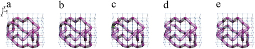
Figure 9. Constructions from figure-8 knot to unknot in the lattices. From (a)–(e), the figure-8 knot changes to unknot. Red (blue) cylinders represent the coupling strengths t = 0.01 (s = 1). Red spheres in the lattices are the sites occupied by the localized eigenstates. These red spheres are connected in purple tubes.
Download figure:
Standard image High-resolution imageRed spheres in figure 9 represent the sites occupied by the localized eigenstates. We can find that for the first figure-8 knot (figure 9(a)), the third structure (figure 9(c)) and the fifth unknot (figure 9(e)), the coordinates of sites occupied by the localized eigenstates are exactly those presented in table 5; but for the second (figure 9(b)) and fourth (figure 9(d)) structures, some sites with coordinates shown in table 5 are not occupied by localized eigenstates. This phenomenon corresponds to the description of changing one crossing in the text around figure 6.
Similar to the electric realization above, we connect every two nearest neighboring nodes in the electric circuit through the capacitors, and the nodes with the coordinates presented in table 5 are connected by small capacitors C1 = 100 pF. Other nodes are connected by large capacitors C2 = 10 nF. Consider the correspondence between the lattice and the electric circuit, we only need to change some capacitors and their associated grounding inductors at each step. In figure 10, we provide the distributions of impedances. We can find that for the first figure-8 knot (figure 10(a)), the third structure (figure 10(c)) and the fifth unknot (figure 10(e)), the coordinates of nodes possessing large impedance are exactly those presented in table 5; but for the second (figure 10(b)) and fourth (figure 10(d)) structures, some sites with coordinates shown in table 5 do not have large impedances, and the connections are broken apart. This corresponds to the observation of localization of eigenstates in the lattices in figure 9.

Figure 10. Simulated distributions of impedance for the five structures from figure-8 knot to unknot. From (a)–(e), the value of impedance at each node has been normalized to the maximum value.
Download figure:
Standard image High-resolution imageD.3. 83 knot
To show the change process that changes from 83 knot to unknot, we need to change crossing in 83 knot twice. The Hamiltonian to realize the change from the 83 knot to unknot in lattice is shown as

Here, we do not provide the details of functions for these structures from the 83 knot to unknot. Consider the coordinates in the lattices are integers, we only provide the integral coordinates satisfying the corresponding functions in tables 6 and 7. To realize the construction of 83 knot to unknot, we show the coordinates in table 6 that connect with the six adjacent sites through the coupling strength ti,j = 0.01 for the first five structures in figure 11, and the coupling strengths between other sites are sk,l = 1. When obtaining the fifth structure, we have changed the crossing in the 83 knot once. At this time, the obtained fifth structure is still knotted.
Table 6. The coordinates  connect with all adjacent sites through ti,j
= 0.01.
connect with all adjacent sites through ti,j
= 0.01.
| The first structure (83 knot) in figure 11(a) | ||||||||||
| (2,4,2) | (3,5,2) | (2,6,2) | (3,7,2) | (2,8,2) | (3,9,2) | (2,10,2) | (3,11,2) | (2,12,2) | (3,13,2) | (2,14,2) |
| (2,15,3) | (2,16,2) | (3,17,2) | (4,18,2) | (4,19,1) | (5,20,1) | (6,20,2) | (7,20,3) | (8,19,3) | (8,18,2) | (9,18,1) |
| (10,17,1) | (10,16,2) | (10,15,3) | (10,14,2) | (9,13,2) | (10,12,2) | (9,11,2) | (10,10,2) | (9,9,2) | (10,8,2) | (9,7,2) |
| (10,6,2) | (9,5,2) | (10,4,2) | (9,3,2) | (8,2,2) | (7,2,3) | (6,3,3) | (5,4,3) | (5,5,2) | (5,6,1) | (6,7,1) |
| (7,8,1) | (7,9,2) | (7,10,3) | (6,11,3) | (5,12,3) | (5,13,2) | (5,14,1) | (6,15,1) | (7,16,1) | (8,16,2) | (8,17,3) |
| (9,18,3) | (10,19,3) | (10,20,2) | (9,21,2) | (8,20,2) | (7,19,2) | (6,18,2) | (5,19,2) | (4,20,2) | (3,21,2) | (2,20,2) |
| (2,19,1) | (3,18,1) | (4,17,1) | (4,16,2) | (5,16,3) | (6,15,3) | (7,14,3) | (7,13,2) | (7,12,1) | (6,11,1) | (5,10,1) |
| (5,9,2) | (5,8,3) | (6,7,3) | (7,6,3) | (7,5,2) | (7,4,1) | (6,3,1) | (5,2,1) | (4,2,2) | (3,3,2) | |
| The second structure in figure 11(b) | ||||||||||
| (2,4,2) | (3,5,2) | (2,6,2) | (3,7,2) | (2,8,2) | (3,9,2) | (2,10,2) | (3,11,2) | (2,12,2) | (3,13,2) | (2,14,2) |
| (2,15,3) | (2,16,2) | (3,17,2) | (4,18,2) | (4,19,1) | (5,20,1) | (6,20,2) | (7,20,3) | (8,19,3) | (8,18,2) | (9,18,1) |
| (10,17,1) | (10,16,2) | (10,15,3) | (10,14,2) | (9,13,2) | (10,12,2) | (9,11,2) | (10,10,2) | (9,9,2) | (10,8,2) | (9,7,2) |
| (10,6,2) | (9,5,2) | (10,4,2) | (9,3,2) | (8,2,2) | (7,2,3) | (6,3,3) | (5,4,3) | (5,5,2) | (5,6,1) | (6,7,1) |
| (7,8,1) | (7,9,2) | (7,10,3) | (6,11,3) | (5,12,3) | (5,13,2) | (5,14,2) | (6,15,2) | (7,16,2) | (8,16,2) | (8,17,3) |
| (9,18,3) | (10,19,3) | (10,20,2) | (9,21,2) | (8,20,2) | (7,19,2) | (6,18,2) | (5,19,2) | (4,20,2) | (3,21,2) | (2,20,2) |
| (2,19,1) | (3,18,1) | (4,17,1) | (4,16,2) | (5,16,3) | (6,15,3) | (7,14,3) | (7,13,2) | (7,12,1) | (6,11,1) | (5,10,1) |
| (5,9,2) | (5,8,3) | (6,7,3) | (7,6,3) | (7,5,2) | (7,4,1) | (6,3,1) | (5,2,1) | (4,2,2) | (3,3,2) | |
| The third structure in figure 11(c) | ||||||||||
| (2,4,2) | (3,5,2) | (2,6,2) | (3,7,2) | (2,8,2) | (3,9,2) | (2,10,2) | (3,11,2) | (2,12,2) | (3,13,2) | (2,14,2) |
| (2,15,3) | (2,16,2) | (3,17,2) | (4,18,2) | (4,19,1) | (5,20,1) | (6,20,2) | (7,20,3) | (8,19,3) | (8,18,2) | (9,18,1) |
| (10,17,1) | (10,16,2) | (10,15,3) | (10,14,2) | (9,13,2) | (10,12,2) | (9,11,2) | (10,10,2) | (9,9,2) | (10,8,2) | (9,7,2) |
| (10,6,2) | (9,5,2) | (10,4,2) | (9,3,2) | (8,2,2) | (7,2,3) | (6,3,3) | (5,4,3) | (5,5,2) | (5,6,1) | (6,7,1) |
| (7,8,1) | (7,9,2) | (7,10,3) | (6,11,3) | (5,12,3) | (5,13,2) | (5,14,3) | (6,15,3) | (7,16,3) | (8,16,2) | (8,17,3) |
| (9,18,3) | (10,19,3) | (10,20,2) | (9,21,2) | (8,20,2) | (7,19,2) | (6,18,2) | (5,19,2) | (4,20,2) | (3,21,2) | (2,20,2) |
| (2,19,1) | (3,18,1) | (4,17,1) | (4,16,2) | (5,16,3) | (6,15,3) | (7,14,3) | (7,13,2) | (7,12,1) | (6,11,1) | (5,10,1) |
| (5,9,2) | (5,8,3) | (6,7,3) | (7,6,3) | (7,5,2) | (7,4,1) | (6,3,1) | (5,2,1) | (4,2,2) | (3,3,2) | |
| The fourth structure in figure 11(d) | ||||||||||
| (2,4,2) | (3,5,2) | (2,6,2) | (3,7,2) | (2,8,2) | (3,9,2) | (2,10,2) | (3,11,2) | (2,12,2) | (3,13,2) | (2,14,2) |
| (2,15,3) | (2,16,2) | (3,17,2) | (4,18,2) | (4,19,1) | (5,20,1) | (6,20,2) | (7,20,3) | (8,19,3) | (8,18,2) | (9,18,1) |
| (10,17,1) | (10,16,2) | (10,15,3) | (10,14,2) | (9,13,2) | (10,12,2) | (9,11,2) | (10,10,2) | (9,9,2) | (10,8,2) | (9,7,2) |
| (10,6,2) | (9,5,2) | (10,4,2) | (9,3,2) | (8,2,2) | (7,2,3) | (6,3,3) | (5,4,3) | (5,5,2) | (5,6,1) | (6,7,1) |
| (7,8,1) | (7,9,2) | (7,10,3) | (6,11,3) | (5,12,3) | (5,13,2) | (5,14,3) | (6,15,3) | (7,16,3) | (8,16,2) | (8,17,3) |
| (9,18,3) | (10,19,3) | (10,20,2) | (9,21,2) | (8,20,2) | (7,19,2) | (6,18,2) | (5,19,2) | (4,20,2) | (3,21,2) | (2,20,2) |
| (2,19,1) | (3,18,1) | (4,17,1) | (4,16,2) | (5,16,2) | (6,15,2) | (7,14,2) | (7,13,2) | (7,12,1) | (6,11,1) | (5,10,1) |
| (5,9,2) | (5,8,3) | (6,7,3) | (7,6,3) | (7,5,2) | (7,4,1) | (6,3,1) | (5,2,1) | (4,2,2) | (3,3,2) | |
| The fifth structure in figure 11(e) | ||||||||||
| (2,4,2) | (3,5,2) | (2,6,2) | (3,7,2) | (2,8,2) | (3,9,2) | (2,10,2) | (3,11,2) | (2,12,2) | (3,13,2) | (2,14,2) |
| (2,15,3) | (2,16,2) | (3,17,2) | (4,18,2) | (4,19,1) | (5,20,1) | (6,20,2) | (7,20,3) | (8,19,3) | (8,18,2) | (9,18,1) |
| (10,17,1) | (10,16,2) | (10,15,3) | (10,14,2) | (9,13,2) | (10,12,2) | (9,11,2) | (10,10,2) | (9,9,2) | (10,8,2) | (9,7,2) |
| (10,6,2) | (9,5,2) | (10,4,2) | (9,3,2) | (8,2,2) | (7,2,3) | (6,3,3) | (5,4,3) | (5,5,2) | (5,6,1) | (6,7,1) |
| (7,8,1) | (7,9,2) | (7,10,3) | (6,11,3) | (5,12,3) | (5,13,2) | (5,14,3) | (6,15,3) | (7,16,3) | (8,16,2) | (8,17,3) |
| (9,18,3) | (10,19,3) | (10,20,2) | (9,21,2) | (8,20,2) | (7,19,2) | (6,18,2) | (5,19,2) | (4,20,2) | (3,21,2) | (2,20,2) |
| (2,19,1) | (3,18,1) | (4,17,1) | (4,16,2) | (5,16,1) | (6,15,1) | (7,14,1) | (7,13,2) | (7,12,1) | (6,11,1) | (5,10,1) |
| (5,9,2) | (5,8,3) | (6,7,3) | (7,6,3) | (7,5,2) | (7,4,1) | (6,3,1) | (5,2,1) | (4,2,2) | (3,3,2) |
Table 7. The coordinates  connect with all adjacent sites through ti,j
= 0.01.
connect with all adjacent sites through ti,j
= 0.01.
| The sixth structure in figure 11(f) | ||||||||||
| (2,4,2) | (3,5,2) | (2,6,2) | (3,7,2) | (2,8,2) | (3,9,2) | (2,10,2) | (3,11,2) | (2,12,2) | (3,13,2) | (2,14,2) |
| (2,15,3) | (2,16,2) | (3,17,2) | (4,18,2) | (4,19,1) | (5,20,1) | (6,20,2) | (7,20,3) | (8,19,3) | (8,18,2) | (9,18,1) |
| (10,17,1) | (10,16,2) | (10,15,3) | (10,14,2) | (9,13,2) | (10,12,2) | (9,11,2) | (10,10,2) | (9,9,2) | (10,8,2) | (9,7,2) |
| (10,6,2) | (9,5,2) | (10,4,2) | (9,3,2) | (8,2,2) | (7,2,3) | (6,3,3) | (5,4,3) | (5,5,2) | (5,6,1) | (6,7,1) |
| (7,8,1) | (7,9,2) | (7,10,3) | (6,11,3) | (5,12,3) | (5,13,2) | (5,14,3) | (6,15,3) | (7,16,3) | (8,16,2) | (8,17,3) |
| (9,18,3) | (10,19,3) | (10,20,2) | (9,21,2) | (8,20,2) | (7,19,2) | (6,18,2) | (5,19,2) | (4,20,2) | (3,21,2) | (2,20,2) |
| (2,19,1) | (3,18,1) | (4,17,1) | (4,16,2) | (5,16,1) | (6,15,1) | (7,14,1) | (7,13,2) | (7,12,1) | (6,11,1) | (5,10,1) |
| (5,9,2) | (5,8,2) | (6,7,2) | (7,6,2) | (7,5,2) | (7,4,1) | (6,3,1) | (5,2,1) | (4,2,2) | (3,3,2) | |
| The seventh structure in figure 11(g) | ||||||||||
| (2,4,2) | (3,5,2) | (2,6,2) | (3,7,2) | (2,8,2) | (3,9,2) | (2,10,2) | (3,11,2) | (2,12,2) | (3,13,2) | (2,14,2) |
| (2,15,3) | (2,16,2) | (3,17,2) | (4,18,2) | (4,19,1) | (5,20,1) | (6,20,2) | (7,20,3) | (8,19,3) | (8,18,2) | (9,18,1) |
| (10,17,1) | (10,16,2) | (10,15,3) | (10,14,2) | (9,13,2) | (10,12,2) | (9,11,2) | (10,10,2) | (9,9,2) | (10,8,2) | (9,7,2) |
| (10,6,2) | (9,5,2) | (10,4,2) | (9,3,2) | (8,2,2) | (7,2,3) | (6,3,3) | (5,4,3) | (5,5,2) | (5,6,1) | (6,7,1) |
| (7,8,1) | (7,9,2) | (7,10,3) | (6,11,3) | (5,12,3) | (5,13,2) | (5,14,3) | (6,15,3) | (7,16,3) | (8,16,2) | (8,17,3) |
| (9,18,3) | (10,19,3) | (10,20,2) | (9,21,2) | (8,20,2) | (7,19,2) | (6,18,2) | (5,19,2) | (4,20,2) | (3,21,2) | (2,20,2) |
| (2,19,1) | (3,18,1) | (4,17,1) | (4,16,2) | (5,16,1) | (6,15,1) | (7,14,1) | (7,13,2) | (7,12,1) | (6,11,1) | (5,10,1) |
| (5,9,2) | (5,8,1) | (6,7,1) | (7,6,1) | (7,5,2) | (7,4,1) | (6,3,1) | (5,2,1) | (4,2,2) | (3,3,2) | |
| The eighth structure in figure 11(h) | ||||||||||
| (2,4,2) | (3,5,2) | (2,6,2) | (3,7,2) | (2,8,2) | (3,9,2) | (2,10,2) | (3,11,2) | (2,12,2) | (3,13,2) | (2,14,2) |
| (2,15,3) | (2,16,2) | (3,17,2) | (4,18,2) | (4,19,1) | (5,20,1) | (6,20,2) | (7,20,3) | (8,19,3) | (8,18,2) | (9,18,1) |
| (10,17,1) | (10,16,2) | (10,15,3) | (10,14,2) | (9,13,2) | (10,12,2) | (9,11,2) | (10,10,2) | (9,9,2) | (10,8,2) | (9,7,2) |
| (10,6,2) | (9,5,2) | (10,4,2) | (9,3,2) | (8,2,2) | (7,2,3) | (6,3,3) | (5,4,3) | (5,5,2) | (5,6,2) | (6,7,2) |
| (7,8,2) | (7,9,2) | (7,10,3) | (6,11,3) | (5,12,3) | (5,13,2) | (5,14,3) | (6,15,3) | (7,16,3) | (8,16,2) | (8,17,3) |
| (9,18,3) | (10,19,3) | (10,20,2) | (9,21,2) | (8,20,2) | (7,19,2) | (6,18,2) | (5,19,2) | (4,20,2) | (3,21,2) | (2,20,2) |
| (2,19,1) | (3,18,1) | (4,17,1) | (4,16,2) | (5,16,1) | (6,15,1) | (7,14,1) | (7,13,2) | (7,12,1) | (6,11,1) | (5,10,1) |
| (5,9,2) | (5,8,1) | (6,7,1) | (7,6,1) | (7,5,2) | (7,4,1) | (6,3,1) | (5,2,1) | (4,2,2) | (3,3,2) | |
| The ninth structure in figure 11(i) | ||||||||||
| (2,4,2) | (3,5,2) | (2,6,2) | (3,7,2) | (2,8,2) | (3,9,2) | (2,10,2) | (3,11,2) | (2,12,2) | (3,13,2) | (2,14,2) |
| (2,15,3) | (2,16,2) | (3,17,2) | (4,18,2) | (4,19,1) | (5,20,1) | (6,20,2) | (7,20,3) | (8,19,3) | (8,18,2) | (9,18,1) |
| (10,17,1) | (10,16,2) | (10,15,3) | (10,14,2) | (9,13,2) | (10,12,2) | (9,11,2) | (10,10,2) | (9,9,2) | (10,8,2) | (9,7,2) |
| (10,6,2) | (9,5,2) | (10,4,2) | (9,3,2) | (8,2,2) | (7,2,3) | (6,3,3) | (5,4,3) | (5,5,2) | (5,6,3) | (6,7,3) |
| (7,8,3) | (7,9,2) | (7,10,3) | (6,11,3) | (5,12,3) | (5,13,2) | (5,14,3) | (6,15,3) | (7,16,3) | (8,16,2) | (8,17,3) |
| (9,18,3) | (10,19,3) | (10,20,2) | (9,21,2) | (8,20,2) | (7,19,2) | (6,18,2) | (5,19,2) | (4,20,2) | (3,21,2) | (2,20,2) |
| (2,19,1) | (3,18,1) | (4,17,1) | (4,16,2) | (5,16,1) | (6,15,1) | (7,14,1) | (7,13,2) | (7,12,1) | (6,11,1) | (5,10,1) |
| (5,9,2) | (5,8,1) | (6,7,1) | (7,6,1) | (7,5,2) | (7,4,1) | (6,3,1) | (5,2,1) | (4,2,2) | (3,3,2) |

Figure 11. Constructions from 83 knot to unknot in the lattices. From (a)–(i), the 83 knot changes to unknot. Red (blue) cylinders represent the coupling strengths t = 0.01 (s = 1). (a)–(e) The first change of the crossing emerges in the 83 knot. (e)–(i) The second change of the crossing emerges in the 83 knot. Red spheres in the lattices are the sites occupied by the localized eigenstates. These red spheres are connected in purple tubes.
Download figure:
Standard image High-resolution imageWhen compared with the chosen coordinates to realize the five structures in the lattices, in table 6, we find that the coordinates from the first to the fifth structure are changed as: first (figure 11(a)) → second (figure 11(b)), (5,14,1) → (5,14,2), (6,15,1) → (6,15,2), (7,16,1) → (7,16,2); second (figure 11(b)) → third (figure 11(c)), (5,14,2) → (5,14,3), (6,15,2) → (6,15,3), (7,16,2) → (7,16,3); third (figure 11(c)) → fourth (figure 11(d)), (5,16,3) → (5,16,2), (6,15,3) → (6,15,2), (7,14,3) → (7,14,2); and fourth (figure 11(d)) → fifth (figure 11(e)), (5,16,2) → (5,16,1), (6,15,2) → (6,15,1), (7,14,2) → (7,14,1). In the change process, only three sites coupled to neighboring sites by strength ti,j = 0.01 are changed and these sites are the nearest neighboring to each other at any two adjacent steps. In this sense, we can view this change process continuously. It means that we need only continuously to modulate three coupling strengths at each step in the change process.
Red spheres in figure 11 represent the sites occupied by the localized eigenstates. We can find that for the first 83 knot (figure 11(a)), the third structure (figure 11(c)) and the fifth structure (figure 11(e)), the coordinates of sites occupied by the localized eigenstates are exactly those presented in table 6; but for the second (figure 11(b)) and fourth (figure 11(d)) structures, some sites with coordinates shown in table 6 are not occupied by localized eigenstates. The change from figures 11(a)–(e) corresponds to the description of changing one crossing in the text around figure 6.
Then we show the coordinates in table 7 that connect with the six adjacent sites through the coupling strength ti,j = 0.01 for the remaining four structures in figure 11 (figures 11(f)–(i)), and the coupling strengths between other sites are sk,l = 1.
When compared with the chosen coordinates to realize from the fifth to the ninth structures in the lattices, in table 7, we find that the coordinates from the fifth to the ninth structures are changed as: fifth (figure 11(e)) → sixth (figure 11(f)), (5,8,3) → (5,8,2), (6,7,3) → (6,7,2), (7,6,3) → (7,6,2); sixth (figure 11(f)) → seventh (figure 11(g)), (5,8,2) → (5,8,1), (6,7,2) → (6,7,1), (7,6,2) → (7,6,1); seventh (figure 11(g)) → eighth (figure 11(h)), (5,6,1) → (5,6,2), (6,7,1) → (6,7,2), (7,8,1) → (7,8,2); and eighth (figure 11(h)) → ninth (figure 11(i)), (5,6,2) → (5,6,3), (6,7,2) → (6,7,3), (7,8,2) → (7,8,3). In the change process, only three sites coupled to neighboring sites by strength ti,j = 0.01 are changed and these sites are the nearest neighboring to each other at any two adjacent steps. In this sense, we can view this change process continuously. It means that we need only continuously to modulate three coupling strengths at each step in the change process. We can find that for the seventh structure (figure 11(g)) and the ninth structure (figure 11(i)), the coordinates of sites occupied by the localized eigenstates are exactly those presented in table 7; but for the sixth (figure 11(f)) and eighth (figure 11(h)) structures, some sites with coordinates shown in table 7 are not occupied by localized eigenstates. The change from figures 11(e)–(i) corresponds to the description of changing one crossing in the text around figure 6. Considering the change process making the 83 knot to unknot, we have gone through the change of crossings twice. So the unknotting number for the 83 knot is two.
Similar to the electric realization above, we connect every two nearest neighboring nodes in the electric circuit through the capacitors, and the nodes with the coordinates presented in tables 6 and 7 are connected by small capacitors C1 = 100 pF. Other nodes are connected by large capacitors C2 = 10 nF. Consider the correspondence between the lattice and the electric circuit, we only need to change some capacitors and their associated grounding inductors at each step. In figure 12, we provide the distributions of impedances. We can find that for the first five structures, the coordinates of nodes possessing large impedance in the 83 knot, the third structure and the fifth unknot are exactly those presented in table 6; but in the second and fourth structures, some sites with coordinates shown in table 6 do not have large impedances. This phenomenon corresponds to the description of changing one crossing in the text around figure 6. For the remaining four structures, the coordinates of nodes possessing large impedance in the seventh structure and the ninth unknot are exactly those presented in table 7; but in the sixth and eighth structures, some sites with coordinates shown in table 7 do not have large impedances. This phenomenon also corresponds to the description of changing one crossing in the text around figure 6. So we need to change the crossings twice to make the 83 knot become unknot.

Figure 12. Simulated distributions of impedance for the nine structures from 83 knot to unknot. In all panels, the value of impedances at each node has been normalized to the maximum impedance. From (a)–(i), the distributions of impedance change from 83 knot to unknot.
Download figure:
Standard image High-resolution imageAppendix E.: The construction details to create electrical knots and links under the action of topoisomerase
E.1. The change from an unknot to one hopf link
Here, we describe how to construct knots and links during the action of topoisomerase on the DNA molecules. In figures 3(a) and (d) of the main text, the DNA molecules display the structures of unknot and hopf link. Here, we provide the expression for the structure in figure 3(a) of the main text as
The structure in figure 3(a) is composed of four fitting curves when we set  . The ranges of coordinates are x ∈ [2, 8], y ∈ [2, 16] and z ∈ [1, 3]. The values of a1 to a52 for these four fitting curves are listed below in tables 8 and 9.
Table 8. The coefficients a1 to a52 in the fdeformed-enz. The values outside and inside [*] are the coefficients of the first and second fitting curves, respectively.
| a1 = 0.0366 − 0.0001i [−8.7080 − 0.3527i] | a2 = 0.4897 + 0.0002i [−5.8720 − 0.1232i] |
| a3 = 0.5668 − 0.0004i [−10.9783 + 1.0580i] | a4 = 0.0011 − 0.0000i [1.0279 + 0.1103i] |
| a5 = −0.0136 + 0.0001i [0.5230 − 0.0286i] | a6 = −0.2117 + 0.0001i [−2.4155 + 0.3235i] |
| a7 = −0.0925 − 0.0001i [0.3322 − 0.0014i] | a8 = −0.1305 + 0.0001i [−0.1337 + 0.1088i] |
| a9 = −0.0312 + 0.0001i [5.2207 − 0.5801i] | a10 = 0.0022 + 0.0000i [−0.0003 + 0.0012i] |
| a11 = −0.0023 + 0.0000i [−0.0596 + 0.0011i] | a12 = 0.0269 + 0.0000i [0.4310 − 0.0472i] |
| a13 = 0.0017 − 0.0000i [0.0320 − 0.0004i] | a14 = 0.0176 − 0.0000i [−0.8800 + 0.0890i] |
| a15 = 0.0316 − 0.0000i [−0.0395 + 0.0045i] | a16 = 0.0092 + 0.0000i [0.0385 + 0.0009i] |
| a17 = 0.0128 − 0.0000i [0.0618 − 0.0027i] | a18 = 9.78 × 10⁻⁴ − 1.77 × 10⁻⁵i [−0.1664 + 0.0109i] |
| a19 = −0.0021 − 0.0000i [0.7112 − 0.1040i] | a20 = −5.32 × 10⁻⁴ − 3.91 × 10⁻⁸i [−0.0142 − 0.0001i] |
| a21 = 4.24 × 10⁻⁴ − 1.29 × 10⁻⁷i [0.0223 − 0.0007i] | a22 = −0.0019 − 0.0000i [0.0269 − 0.0011i] |
| a23 = −1.18 × 10⁻⁴ + 1.67 × 10⁻⁷i [−0.0099 + 0.0000i] | a24 = −0.0026 − 0.0000i [−0.0155 − 0.0044i] |
| a25 = −6.10 × 10⁻⁴ + 1.92 × 10⁻⁶i [0.0248 + 0.0004i] | a26 = −1.28 × 10⁻⁶ + 2.36 × 10⁻⁷i [−0.0011 + 0.0002i] |
| a27 = −0.0013 + 0.0000i [0.0165 − 0.0016i] | a28 = −0.0017 + 0.0000i [0.0352 − 0.0033i] |
| a29 = −2.83 × 10⁻⁴ + 2.53 × 10⁻⁶i [−0.0212 + 0.0006i] | a30 = −5.13 × 10⁻⁴ − 4.61 × 10⁻⁷i [1.91 × 10⁻⁴ + 1.33 × 10⁻⁵i] |
| a31 = −7.29 × 10⁻⁴ − 2.52 × 10⁻⁷i [0.0046 − 0.0018i] | a32 = 2.15 × 10⁻⁴ + 5.36 × 10⁻⁷i [−0.0174 + 0.0030i] |
| a33 = 6.08 × 10⁻⁴ + 3.04 × 10⁻⁷i [−0.0423 + 0.0058i] | a34 = −1.95 × 10⁻⁴ + 5.22 × 10⁻⁹i [−0.1442 + 0.0246i] |
| a35 = −9.21 × 10⁻⁷ − 2.53 × 10⁻¹⁰i [2.61 × 10⁻⁵ − 1.21 × 10⁻⁶i] | a36 = −6.91 × 10⁻⁷ + 2.55 × 10⁻¹⁰i [−4.86 × 10⁻⁵ + 2.31 × 10⁻⁶i] |
| a37 = 2.30 × 10⁻⁸ − 4.41 × 10⁻¹⁰i [1.17 × 10⁻⁵ − 9.81 × 10⁻⁷i] | a38 = −1.77 × 10⁻⁷ + 3.66 × 10⁻¹¹i [1.17 × 10⁻⁵ − 1.23 × 10⁻⁷i] |
| a39 = 1.04 × 10⁻⁴ + 4.87 × 10⁻⁸i [−0.0020 + 0.0003i] | a40 = 1.12 × 10⁻⁴ + 2.94 × 10⁻⁸i [−0.0017 + 0.0004i] |
| a41 = 1.98 × 10⁻⁵ + 7.43 × 10⁻⁹i [−3.44 × 10⁻⁴ + 8.24 × 10⁻⁵i] | a42 = −2.28 × 10⁻⁶ + 3.71 × 10⁻⁹i [−4.78 × 10⁻⁵ + 3.00 × 10⁻⁷i] |
| a43 = 6.77 × 10⁻⁶ − 1.13 × 10⁻⁸i [4.52 × 10⁻⁵ − 7.48 × 10⁻⁶i] | a44 = −1.92 × 10⁻⁷ − 5.90 × 10⁻¹⁰i [2.02 × 10⁻⁵ − 3.70 × 10⁻⁶i] |
| a45 = 5.63 × 10⁻⁵ − 2.93 × 10⁻⁷i [0.0039 − 0.0005i] | a46 = −3.05 × 10⁻⁵ − 1.88 × 10⁻⁸i [0.0025 − 0.0003i] |
| a47 = −7.42 × 10⁻⁶ + 9.20 × 10⁻⁹i [6.30 × 10⁻⁶ + 3.32 × 10⁻⁶i] | a48 = −5.48 × 10⁻⁹ + 7.95 × 10⁻¹⁰i [−6.25 × 10⁻⁵ + 7.69 × 10⁻⁶i] |
| a49 = 5.98 × 10⁻⁵ − 1.37 × 10⁻⁷i [0.0214 − 0.0038i] | a50 = −4.29 × 10⁻⁶ + 1.17 × 10⁻⁸i [−0.0015 + 0.0003i] |
| a51 = 3.05 × 10⁻⁵ + 3.57 × 10⁻⁹i [5.73 × 10⁻⁵ − 1.09 × 10⁻⁶i] | a52 = 1.48 × 10⁻⁵ + 7.54 × 10⁻⁹i [−3.43 × 10⁻⁴ − 1.41 × 10⁻⁷i] |
Table 9. The coefficients from a1 to a52 in the fdeformed-enz. The values outside and inside [*] are the coefficients of the third and fourth fitting curves, respectively.
| a1 = 4.8993 − 0.2168i [0.5638 + 0.0000i] | a2 = 0.8923 − 0.0304i [0.1745 − 0.0000i] |
| a3 = −3.0015 + 0.2860i [0.6397 − 0.0000i] | a4 = −0.4972 − 0.0208i [−0.1295 − 0.0000i] |
| a5 = −0.7281 + 0.0383i [−0.0619 − 0.0000i] | a6 = −0.2780 + 0.0531i [−0.3271 + 0.0000i] |
| a7 = 0.0165 + 0.0052i [0.0411 + 0.0000i] | a8 = 0.4229 − 0.0311i [−0.1675 − 0.0000i] |
| a9 = −0.8512 + 0.0344i [−0.0351 − 0.0000i] | a10 = 0.1328 − 0.0019i [0.0145 + 0.0000i] |
| a11 = −0.0088 − 0.0032i [0.0037 + 0.0000i] | a12 = 0.6662 + 0.0227i [0.0706 − 0.0000i] |
| a13 = −0.0093 + 0.0025i [−0.0042 + 0.0000i] | a14 = −0.6444 − 0.0336i [0.0153 + 0.0000i] |
| a15 = −0.2015 + 0.0029i [0.0410 + 0.0000i] | a16 = −0.0105 + 0.0008i [−0.0058 − 0.0000i] |
| a17 = 0.0537 − 0.0098i [−0.0140 + 0.0000i] | a18 = 0.0193 + 0.0375i [0.0429 − 0.0000i] |
| a19 = −0.4823 − 0.0711i [−0.0215 + 0.0000i] | a20 = −0.0130 + 0.0012i [−6.30 × 10⁻⁴ − 1.28 × 10⁻¹¹i] |
| a21 = 0.0010 − 0.0002i [5.42 × 10⁻⁶ + 1.23 × 10⁻¹²i] | a22 = −0.2148 + 0.0068i [−0.0072 + 0.0000i] |
| a23 = −0.0072 − 0.0000i [4.00 × 10⁻⁴ − 9.66 × 10⁻¹²i] | a24 = 0.0345 − 0.0006i [−0.0019 − 0.0000i] |
| a25 = 0.1795 − 0.0200i [−0.0028 − 0.0000i] | a26 = 0.0123 − 0.0002i [4.21 × 10⁻⁶ + 6.45 × 10⁻¹²i] |
| a27 = 0.0205 − 0.0025i [0.0021 − 0.0000i] | a28 = −0.0373 + 0.0047i [−0.0049 + 0.0000i] |
| a29 = 0.0354 + 0.0028i [0.0038 − 0.0000i] | a30 = −0.0031 − 0.0001i [3.64 × 10⁻⁴ + 6.91 × 10⁻¹²i] |
| a31 = 0.0004 − 0.0014i [0.0028 + 0.0000i] | a32 = 0.0070 + 0.0012i [−0.0035 + 0.0000i] |
| a33 = 0.0008 − 0.0027i [−0.0016 − 0.0000i] | a34 = −0.0543 + 0.0089i [0.0020 + 0.0000i] |
| a35 = −2.19 × 10⁻⁵ + 9.23 × 10⁻⁷i [5.14 × 10⁻⁸ − 2.20 × 10⁻¹⁴i] | a36 = −6.65 × 10⁻⁵ − 2.71 × 10⁻⁶i [−1.40 × 10⁻⁸ + 4.01 × 10⁻¹⁵i] |
| a37 = −6.65 × 10⁻⁵ + 2.71 × 10⁻⁶i [1.26 × 10⁻⁹ − 1.39 × 10⁻¹⁴i] | a38 = 2.22 × 10⁻⁵ − 9.03 × 10⁻⁷i [6.90 × 10⁻⁸ + 3.30 × 10⁻¹⁴i] |
| a39 = 0.0131 − 0.0012i [2.73 × 10⁻⁴ − 1.03 × 10⁻¹²i] | a40 = −0.0034 + 0.0002i [−2.84 × 10⁻⁴ + 4.03 × 10⁻¹²i] |
| a41 = −8.45 × 10⁻⁴ + 2.57 × 10⁻⁴i [−1.75 × 10⁻⁴ + 3.72 × 10⁻¹³i] | a42 = 1.63 × 10⁻⁴ + 1.53 × 10⁻⁴i [2.07 × 10⁻⁵ − 4.15 × 10⁻¹⁴i] |
| a43 = 0.0011 − 0.0000i [4.21 × 10⁻⁵ − 1.53 × 10⁻¹³i] | a44 = −9.60 × 10⁻⁵ − 2.49 × 10⁻⁵i [2.87 × 10⁻⁶ − 5.52 × 10⁻¹⁴i] |
| a45 = −0.0323 + 0.0035i [−4.00 × 10⁻⁵ + 1.57 × 10⁻¹²i] | a46 = −3.76 × 10⁻⁴ − 2.47 × 10⁻⁴i [2.05 × 10⁻⁴ + 4.76 × 10⁻¹³i] |
| a47 = 0.0050 − 0.0001i [−4.10 × 10⁻⁵ + 1.22 × 10⁻¹³i] | a48 = 1.26 × 10⁻⁴ + 5.26 × 10⁻⁵i [2.09 × 10⁻⁶ + 2.68 × 10⁻¹⁴i] |
| a49 = 0.0012 − 0.0000i [4.13 × 10⁻⁵ − 5.89 × 10⁻¹²i] | a50 = −5.17 × 10⁻⁵ − 2.67 × 10⁻⁵i [−1.47 × 10⁻⁵ + 4.70 × 10⁻¹³i] |
| a51 = −3.80 × 10⁻⁶ − 3.43 × 10⁻⁷i [−8.81 × 10⁻⁷ + 8.87 × 10⁻¹³i] | a52 = 5.41 × 10⁻⁷ − 4.57 × 10⁻⁸i [−2.22 × 10⁻⁶ − 8.48 × 10⁻¹³i] |
The other structure shown in figure 3(d) can be obtained in functions in the same way, we do not provide functions here for the lengthy expressions. Here we show how to construct these structures in the lattices. These two structures in figures 3(a) and (d) of the main text are constructed in the lattices as,

The site in the lattice is often described by the integral coordinate. Since we have provided the function describing the structure in figure 3(a) as  . The ranges of x, y, z coordinates in the lattice are x ∈ [2, 8], y ∈ [2, 16], z ∈ [1, 3], and the values of x, y, z are all integers. Therefore, to construct this structure in the lattice, we seek all integral coordinates satisfying
  . We list all these coordinates in sequence in table 10 below. In the realization of this structure, the coordinates in table 10 are those connected with the six adjacent sites through the coupling strength ti,j
= 0.01, and the coupling strengths between other sites are sk,l
= 1. Moreover, for the structure in figure 3(d), we also provide the coordinates that connect with the six adjacent sites through the coupling strength ti,j
= 0.01 in table 10, and other sites are connected by sk,l
= 1.
. We list all these coordinates in sequence in table 10 below. In the realization of this structure, the coordinates in table 10 are those connected with the six adjacent sites through the coupling strength ti,j
= 0.01, and the coupling strengths between other sites are sk,l
= 1. Moreover, for the structure in figure 3(d), we also provide the coordinates that connect with the six adjacent sites through the coupling strength ti,j
= 0.01 in table 10, and other sites are connected by sk,l
= 1.
Table 10. The coordinates  connect with all adjacent sites through ti,j
= 0.01.
connect with all adjacent sites through ti,j
= 0.01.
| Figure 3(a) in the main text | |||||||||
| (2,3,2) | (2,4,1) | (3,5,1) | (4,6,1) | (4,7,2) | (4,8,3) | (3,9,3) | (2,10,3) | (2,11,2) | (2,12,1) |
| (3,13,1) | (4,14,1) | (5,14,2) | (6,13,2) | (6,12,1) | (6,11,2) | (7,10,2) | (8,11,2) | (8,12,3) | (8,13,2) |
| (8,14,3) | (7,15,3) | (6,16,3) | (5,16,2) | (4,16,3) | (3,16,2) | (2,15,2) | (2,14,3) | (3,13,3) | (4,12,3) |
| (4,11,2) | (4,10,1) | (3,9,1) | (2,8,1) | (2,7,2) | (2,6,3) | (3,5,3) | (4,4,3) | (5,4,2) | (6,5,2) |
| (6,6,3) | (6,7,2) | (7,8,2) | (8,7,2) | (8,6,1) | (8,5,2) | (8,4,1) | (7,3,1) | (6,2,1) | (5,2,2) |
| (4,2,1) | (3,2,2) | ||||||||
| Figure 3(d) in the main text | |||||||||
| (2,3,2) | (2,4,1) | (3,5,1) | (4,6,1) | (4,7,2) | (4,8,3) | (3,9,3) | (2,10,3) | (2,11,2) | (2,12,1) |
| (3,13,1) | (4,14,1) | (5,14,2) | (6,13,2) | (6,12,1) | (6,11,2) | (6,10,1) | (7,9,1) | (8,8,1) | (8,7,2) |
| (8,6,1) | (8,5,2) | (8,4,1) | (7,3,1) | (6,2,1) | (5,2,2) | (4,2,1) | (3,2,2) | (4,4,3) | (3,5,3) |
| (2,6,3) | (2,7,2) | (2,8,1) | (3,9,1) | (4,10,1) | (4,11,2) | (4,12,3) | (3,13,3) | (2,14,3) | (2,15,2) |
| (3,16,2) | (4,16,3) | (5,16,2) | (6,16,3) | (7,15,3) | (8,14,3) | (8,13,2) | (8,12,3) | (8,11,2) | (8,10,3) |
| (7,9,3) | (6,8,3) | (6,7,2) | (6,6,3) | (6,5,2) | (5,4,2) |
In figures 13(a) and (b), we provide the realizations of such unknot (figure 3(a) of the main text) and hopf link (figure 3(d) of the main text) in the lattices. Red (blue) cylinders in the lattices represent the coupling strengths ti,j = 0.01 (sk,l = 1). Red spheres in the lattices represent the sites occupied by localized eigenstates. As shown in figure 13, these sites are exactly those presented in table 10. To illustrate the distribution clearly, we use the purple and orange tubes in figure 13 to connect these sites. We find that they comprise the unknot and hopf link, respectively. So we realize 'discrete' versions of unknot and hopf link.

Figure 13. Lattices constructions to show the DNA structures of figures 3(a) and (d) in the main text. (a) The unknot in figure 3(a), (b) the hopf link in figure 3(d). In (a) and (b), red (blue) cylinders represent the coupling strengths t = 0.01 (s = 1). Red spheres in the lattices are the sites occupied by the localized eigenstates. We connect these sites through red and orange tubes. (c) The electrically experimental setup to realize these two structures.
Download figure:
Standard image High-resolution imageThe corresponding electric circuits are presented in figure 13(c). Similar to the electric realization above, we connect every two nearest neighboring nodes in the electric circuit through the capacitors. The nodes with the coordinates presented in table 10 are connected by small capacitors C1 = 100 pF, and other nodes are connected by large capacitors C2 = 10 nF. Experimentally measured impedances have been shown in figure 3 of the main text. Although we provide only one experiment setup in figure 13(c), we can only modulate some electric capacitors and associated grounding inductors to accomplish the constructions of these two structures in the circuits.
E.2. The change from the hopf link to the figure-8 knot
Actually, the DNA molecule changes to a new topology (figure-8 knot) if the Tn3 resolvase acts on the DNA molecule with the topology in figure 3(d) of the main text again [1]. Here we will show how to realize these two structures in the lattices, the corresponding electric designs can be realized following the way above. These two structures are constructed in the lattices as,

Here, we do not provide the functions of these two structures for their lengthy expressions. Consider the sites in the lattices are described by the integral coordinates, we provide the coordinates satisfying those functions in table 11. In the realizations of these two structures, the coordinates in table 11 connect with the six adjacent sites through the coupling strength ti,j = 0.01, and the coupling strengths between other sites are sk,l = 1.
Table 11. The coordinates  connect with all adjacent sites through ti,j
= 0.01.
connect with all adjacent sites through ti,j
= 0.01.
| The Tn3 resolvase acts on the DNA molecule once (hopf link) | ||||||||||
| (2,3,2) | (2,4,1) | (3,5,1) | (4,6,1) | (4,7,2) | (4,8,3) | (3,9,3) | (2,10,3) | (2,11,2) | (2,12,1) | (3,13,1) |
| (4,14,1) | (5,14,2) | (6,13,2) | (6,12,1) | (6,11,2) | (7,10,2) | (8,11,2) | (8,12,3) | (8,13,2) | (9,14,2) | (10,13,2) |
| (10,12,1) | (10,11,2) | (10,10,1) | (11,9,1) | (12,8,1) | (12,7,2) | (12,6,1) | (12,5,2) | (12,4,1) | (11,3,1) | (10,2,1) |
| (9,2,2) | (8,2,1) | (7,2,2) | (6,2,1) | (5,2,2) | (4,2,1) | (3,2,2) | (4,4,3) | (3,5,3) | (2,6,3) | (2,7,2) |
| (2,8,1) | (3,9,1) | (4,10,1) | (4,11,2) | (4,12,3) | (3,13,3) | (2,14,3) | (2,15,2) | (3,16,2) | (4,16,3) | (5,16,2) |
| (6,16,3) | (7,16,2) | (8,16,3) | (9,16,2) | (10,16,3) | (11,15,3) | (12,14,3) | (12,13,2) | (12,12,3) | (12,11,2) | (12,10,3) |
| (11,9,3) | (10,8,3) | (10,7,2) | (10,6,3) | (10,5,2) | (9,4,2) | (8,5,2) | (8,6,1) | (8,7,2) | (7,8,2) | (6,7,2) |
| (6,6,3) | (6,5,2) | (5,4,2) | ||||||||
| The Tn3 resolvase acts on the DNA molecule twice (figure-8 knot) | ||||||||||
| (2,3,2) | (2,4,1) | (3,5,1) | (4,6,1) | (4,7,2) | (4,8,3) | (3,9,3) | (2,10,3) | (2,11,2) | (2,12,1) | (3,13,1) |
| (4,14,1) | (5,14,2) | (6,13,2) | (6,12,1) | (6,11,2) | (6,10,1) | (7,9,1) | (8,8,1) | (8,7,2) | (8,6,1) | (8,5,2) |
| (9,4,2) | (10,5,2) | (10,6,3) | (10,7,2) | (10,8,3) | (11,9,3) | (12,10,3) | (12,11,2) | (12,12,3) | (12,13,2) | (12,14,3) |
| (11,15,3) | (10,16,3) | (9,16,2) | (8,16,3) | (7,16,2) | (6,16,3) | (5,16,2) | (4,16,3) | (3,16,2) | (2,15,2) | (2,14,3) |
| (3,13,3) | (4,12,3) | (4,11,2) | (4,10,1) | (3,9,1) | (2,8,1) | (2,7,2) | (2,6,3) | (3,5,3) | (4,4,3) | (5,4,2) |
| (6,5,2) | (6,6,3) | (6,7,2) | (6,8,3) | (7,9,3) | (8,10,3) | (8,11,2) | (8,12,3) | (8,13,2) | (9,14,2) | (10,13,2) |
| (10,12,1) | (10,11,2) | (10,10,1) | (11,9,1) | (12,8,1) | (12,7,2) | (12,6,1) | (12,5,2) | (12,4,1) | (11,3,1) | (10,2,1) |
| (9,2,2) | (8,2,1) | (7,2,2) | (6,2,1) | (5,2,2) | (4,2,1) | (3,2,2) |
In figure 14, we provide the realizations of these two structures in the lattices. Red (blue) cylinders in the lattices represent the coupling strengths ti,j = 0.01 (sk,l = 1).

Figure 14. Constructions in the lattices and simulated distributions of impedance for these two structures in the electric circuits. (a) The structure with the Tn3 resolvase acts on the DNA molecule once (hopf link), (b) the structure with the Tn3 resolvase acts on the DNA molecule twice (figure-8 knot). In (a) and (b), red (blue) cylinders represent the coupling strengths t = 0.01 (s = 1). Red spheres in the lattices are the sites occupied by the localized eigenstates. We connect these sites through red and orange tubes. In (c) and (d), the value of impedance at each node has been normalized to the maximum value.
Download figure:
Standard image High-resolution imageAs shown in figure 14, red spheres in the lattices represent the sites occupied by localized eigenstates. These sites are exactly those presented in table 11. To illustrate the distribution clearly, we use the purple and orange tubes in figure 14 to connect these sites. We find that they comprise the 'discrete' hopf link and figure-8 knot, respectively. The corresponding electric realizations are similar to the above. We connect every two nearest neighboring nodes in the electric circuit through the capacitors. The nodes with the coordinates presented in table 11 are connected by small capacitors C1 = 100 pF, and other nodes are connected by large capacitors C2 = 10 nF. The large impedances will emerge at those nodes exactly presented in table 11.
Appendix F.: Construction details for the DNA structures with different twists and writhes
F.1. Construction details for DNA structures in figures 4(a), (d) and (g)
Here, we describe how to construct DNA structures with different twists and writhes. In figures 4(a), (d) and (g) of the main text, we provide three topologically equivalent structures. The first structure (figure 4(a)) has the twist Tw = 0 and the writhe Wr = 1. The third structure (figure 4(g)) has the twist Tw = 1 and the writhe Wr = 0. The electric realizations of these three structures have been provided in figures 4(b), (e) and (h), respectively. We provide the expression (equation (F1)) for the structure shown in figure 4(a) below,
The structure in figure 4(a) is composed of two fitting curves when we set  . The ranges of coordinates are, x ∈ [3, 11], y ∈ [2, 14], z ∈ [1, 3]. The values of a1 to a52 for these two fitting curves are listed below in table 12.
Table 12. The coefficients a1 to a52 in the fdeformed-link. The values outside and inside [*] are the coefficients of the first and second fitting curves, respectively.
| a1 = 0.0632 − 0.0092i [0.3092 − 0.0595i] | a2 = 0.3050 − 0.0621i [0.0113 − 0.0270i] |
| a3 = 0.7021 + 0.0642i [1.0384 + 0.0997i] | a4 = 0.0099 + 0.0083i [−0.0092 + 0.0238i] |
| a5 = −0.0083 + 0.0029i [−0.0285 − 0.0029i] | a6 = −0.1867 + 0.0176i [−0.1637 + 0.0024i] |
| a7 = −0.0285 + 0.0062i [0.0142 + 0.0015i] | a8 = −0.1283 + 0.0421i [−0.1801 + 0.0755i] |
| a9 = 0.1187 − 0.0650i [0.0505 − 0.1290i] | a10 = 0.0012 − 0.0004i [−0.0041 − 0.0012i] |
| a11 = 0.0029 − 0.0005i [0.0064 − 0.0012i] | a12 = 0.0077 − 0.0079i [0.0003 − 0.0087i] |
| a13 = 0.0017 + 0.0002i [−0.0040 + 0.0013i] | a14 = 0.0139 + 0.0070i [0.0086 − 0.0040i] |
| a15 = 0.0142 − 0.0087i [0.0115 − 0.0101i] | a16 = −0.0008 + 0.0011i [0.0018 + 0.0011i] |
| a17 = 0.0106 − 0.0085i [0.0118 − 0.0091i] | a18 = −0.0263 + 0.0207i [−0.0143 + 0.0193i] |
| a19 = −0.0631 + 0.0161i [−0.1054 + 0.0236i] | a20 = −7.41 × 10⁻⁵ − 6.92 × 10⁻⁵i [4.21 × 10⁻⁴ − 1.15 × 10⁻⁴i] |
| a21 = 1.35 × 10⁻⁴ + 5.29 × 10⁻⁵i [−4.22 × 10⁻⁴ + 4.06 × 10⁻⁵i] | a22 = 1.05 × 10⁻⁴ − 1.20 × 10⁻⁴i [0.0011 + 0.0001i] |
| a23 = 2.21 × 10⁻⁵ + 2.17 × 10⁻⁵i [−1.82 × 10⁻⁴ + 6.95 × 10⁻⁵i] | a24 = 1.19 × 10⁻⁴ + 1.75 × 10⁻⁴i [2.52 × 10⁻⁴ + 9.47 × 10⁻⁴i] |
| a25 = −0.0018 + 0.0005i [−0.0012 + 0.0002i] | a26 = −1.35 × 10⁻⁴ − 5.29 × 10⁻⁵i [4.22 × 10⁻⁴ − 4.06 × 10⁻⁵i] |
| a27 = −3.93 × 10⁻⁴ + 6.74 × 10⁻⁴i [−0.0015 + 0.0002i] | a28 = 0.0011 + 0.0023i [0.0093 + 0.0046i] |
| a29 = 0.0117 − 0.0030i [0.0007 + 0.0033i] | a30 = 1.56 × 10⁻⁴ − 9.24 × 10⁻⁵i [−2.37 × 10⁻⁴ − 9.53 × 10⁻⁵i] |
| a31 = 4.28 × 10⁻⁴ − 8.72 × 10⁻⁴i [0.0001 − 0.0012i] | a32 = −0.0024 + 0.0011i [−0.0052 + 0.0013i] |
| a33 = 0.0110 − 0.0073i [0.0282 − 0.0100i] | a34 = 0.0002 + 0.0010i [0.0149 + 0.0050i] |
| a35 = 1.61 × 10⁻⁷ + 1.38 × 10⁻⁸i [−3.02 × 10⁻⁷ + 1.49 × 10⁻⁸i] | a36 = −4.83 × 10⁻⁷ − 4.15 × 10⁻⁸i [9.08 × 10⁻⁷ − 4.45 × 10⁻⁸i] |
| a37 = 4.83 × 10⁻⁷ + 4.16 × 10⁻⁸i [−9.08 × 10⁻⁷ + 4.45 × 10⁻⁸i] | a38 = −1.61 × 10⁻⁷ − 1.39 × 10⁻⁸i [3.02 × 10⁻⁷ − 1.49 × 10⁻⁸i] |
| a39 = −1.22 × 10⁻⁴ + 1.06 × 10⁻⁴i [−1.98 × 10⁻⁴ + 1.51 × 10⁻⁴i] | a40 = 3.87 × 10⁻⁵ − 2.04 × 10⁻⁵i [2.64 × 10⁻⁴ − 9.22 × 10⁻⁵i] |
| a41 = −5.52 × 10⁻⁵ + 1.01 × 10⁻⁴i [−6.71 × 10⁻⁵ + 1.28 × 10⁻⁴i] | a42 = 4.30 × 10⁻⁵ − 2.25 × 10⁻⁵i [7.05 × 10⁻⁵ − 2.08 × 10⁻⁵i] |
| a43 = −2.10 × 10⁻⁵ − 1.22 × 10⁻⁵i [−1.17 × 10⁻⁴ − 1.54 × 10⁻⁵i] | a44 = 1.27 × 10⁻⁵ − 1.19 × 10⁻⁵i [4.64 × 10⁻⁵ − 1.06 × 10⁻⁵i] |
| a45 = −0.0011 + 0.0001i [−0.0013 − 0.0009i] | a46 = 1.64 × 10⁻⁴ − 6.35 × 10⁻⁵i [−0.0013 + 0.0002i] |
| a47 = −8.66 × 10⁻⁵ + 4.50 × 10⁻⁵i [−1.40 × 10⁻⁴ + 4.15 × 10⁻⁵i] | a48 = −1.55 × 10⁻⁴ + 7.62 × 10⁻⁵i [−2.22 × 10⁻⁴ − 1.38 × 10⁻⁵i] |
| a49 = 0.0013 − 0.0003i [0.0015 + 0.0008i] | a50 = 4.33 × 10⁻⁵ − 2.25 × 10⁻⁵i [6.98 × 10⁻⁵ − 2.08 × 10⁻⁵i] |
| a51 = 4.24 × 10⁻¹⁰ − 3.53 × 10⁻¹¹i [−8.44 × 10⁻⁹ − 1.73 × 10⁻⁹i] | a52 = −1.43 × 10⁻⁹ + 5.37 × 10⁻¹⁰i [6.21 × 10⁻⁹ + 1.35 × 10⁻⁹i] |
Other structures shown in figures 4(d) and (g) can be obtained in functions in the same way, and we do not provide the detailed lengthy expressions here. Then we show how to construct these structures in the lattices. These three structures in figure 4 of the main text are constructed in the lattices as,

The site in the lattice is often described by the integral coordinate. Since we have provided the function describing the structure in figure 4(a) as  . The ranges of x, y, z coordinates in the lattice are x ∈ [3, 11], y ∈ [2, 14], z ∈ [1, 3], and the values of x, y, z are all integers. Therefore, to construct this structure in the lattice, we seek all integral coordinates satisfying
  . We list all these coordinates in sequence in table 13 below. In the realization of this structure, these coordinates connecting with the six adjacent sites through the coupling strength ti,j
= 0.01, and the coupling strengths between other sites are sk,l
= 1. Moreover, for the structures in figures 4(d) and (g), we also provide the coordinates connecting with the six adjacent sites through the coupling strength ti,j
= 0.01 in table 13.
. We list all these coordinates in sequence in table 13 below. In the realization of this structure, these coordinates connecting with the six adjacent sites through the coupling strength ti,j
= 0.01, and the coupling strengths between other sites are sk,l
= 1. Moreover, for the structures in figures 4(d) and (g), we also provide the coordinates connecting with the six adjacent sites through the coupling strength ti,j
= 0.01 in table 13.
Table 13. The coordinates  connect with all adjacent sites through ti,j
= 0.01.
connect with all adjacent sites through ti,j
= 0.01.
| The structure in figure 4(a) of the main text | ||||||||||
| (3,5,1) | (4,6,1) | (5,7,1) | (6,8,1) | (7,9,1) | (8,10,1) | (9,11,1) | (8,12,1) | (7,12,2) | (6,12,3) | (5,11,3) |
| (6,10,3) | (7,9,3) | (8,8,3) | (9,7,3) | (10,6,3) | (11,5,3) | (10,4,3) | (9,3,3) | (8,2,3) | (7,2,2) | (6,2,1) |
| (5,3,1) | (4,4,1) | (5,5,1) | (6,6,1) | (7,7,1) | (8,8,1) | (9,9,1) | (10,10,1) | (11,11,1) | (10,12,1) | (9,13,1) |
| (8,14,1) | (7,14,2) | (6,14,3) | (5,13,3) | (4,12,3) | (3,11,3) | (4,10,3) | (5,9,3) | (6,8,3) | (7,7,3) | (8,6,3) |
| (9,5,3) | (8,4,3) | (7,4,2) | (6,4,1) | |||||||
| The structure in figure 4(d) of the main text | ||||||||||
| (2,6,2) | (2,7,1) | (2,8,2) | (2,9,1) | (2,10,2) | (3,11,2) | (4,11,1) | (5,11,2) | (6,11,1) | (7,11,2) | (7,12,3) |
| (6,12,4) | (7,11,4) | (8,11,5) | (9,11,4) | (10,11,5) | (11,11,4) | (12,10,4) | (12,9,5) | (12,8,4) | (12,7,5) | (12,6,4) |
| (11,5,4) | (10,4,4) | (9,3,4) | (8,2,4) | (7,2,3) | (6,2,2) | (5,3,2) | (4,4,2) | (3,5,2) | (4,6,2) | (4,7,1) |
| (4,8,2) | (4,9,1) | (5,9,2) | (6,9,1) | (7,9,2) | (8,9,1) | (9,10,1) | (10,11,1) | (10,12,2) | (9,13,2) | (8,14,2) |
| (7,14,3) | (6,14,4) | (5,13,4) | (4,12,4) | (4,11,5) | (4,10,4) | (5,9,4) | (6,9,5) | (7,9,4) | (8,9,5) | (9,9,4) |
| (10,9,5) | (10,8,4) | (10,7,5) | (10,6,4) | (9,5,4) | (8,4,4) | (7,4,3) | (6,4,2) | (5,5,2) | ||
| The structure in figure 4(g) of the main text | ||||||||||
| (2,6,2) | (2,7,1) | (2,8,2) | (2,9,1) | (2,10,2) | (3,11,2) | (4,11,1) | (5,11,2) | (6,11,1) | (7,11,2) | (7,12,3) |
| (8,12,4) | (9,11,4) | (10,10,4) | (11,10,3) | (12,9,3) | (12,8,4) | (12,7,5) | (12,6,4) | (11,5,4) | (10,4,4) | (9,3,4) |
| (8,2,4) | (7,2,3) | (6,2,2) | (5,3,2) | (4,4,2) | (3,5,2) | (4,6,2) | (4,7,1) | (4,8,2) | (4,9,1) | (5,9,2) |
| (6,9,1) | (7,9,2) | (8,9,1) | (9,10,1) | (10,11,1) | (10,12,2) | (9,13,2) | (8,13,1) | (8,14,2) | (9,14,3) | (10,14,4) |
| (11,14,5) | (12,13,5) | (12,12,4) | (12,11,5) | (11,10,5) | (10,9,5) | (10,8,4) | (10,7,5) | (10,6,4) | (9,5,4) | (8,4,4) |
| (7,4,3) | (6,4,2) | (5,5,2) |
In figures 15(a)–(c), we provide the realizations of these three structures in the lattices. Red (blue) cylinders in the lattices represent the coupling strengths ti,j = 0.01 (sk,l = 1). Red spheres in the lattices represent the sites occupied by localized eigenstates. As shown in figures 15(a)–(c), these sites are exactly those presented in table 13. To illustrate the distribution clearly, we use the purple and orange tubes in figures 15(a)–(c) to connect these sites. We find that they comprise the first structure with the twist Tw = 0 and the writhe Wr = 1 (figure 15(a)), the second structure (figure 15(b)) and the third structure with the twist Tw = 1 and the writhe Wr = 0 (figure 15(c)), respectively. So we realize 'discrete' versions of three structures in figures 4(a), (d) and (g) of the main text.

Figure 15. Constructions of DNA structures with three different geometries in the lattices. (a) The twist Tw = 0 and the writhe Wr = 1, same as that presented in figure 4(a) of the main text. (b) Same as in figure 4(d) of the main text. (c) The twist Tw = 1 and the writhe Wr = 0, same as in figure 4(g) of the main text. In (a)–(c), red (blue) cylinders represent the coupling strengths t = 0.01 (s = 1). Red spheres denote the sites occupied by localized eigenstates. We connect these sites in one purple and orange tubes. (d) The corresponding electrically experimental setup to realize these three structures.
Download figure:
Standard image High-resolution imageThe corresponding electric circuits are also presented in figure 15(d). Similar to the electric realization above, we connect every two nodes in the electric circuit through the capacitors. The nodes with the coordinates presented in table 13 are connected by C1 = 100 pF, and other nodes are connected by C2 = 10 nF. The corresponding experimental designs have been provided in figures 4(b), (e) and (h) of the main text, respectively. Experimentally measured impedances in these circuits have been shown in figures 4(c), (f) and (i) of the main text, respectively.
F.2. Construction details of DNA structures in the middle of change process
To demonstrate these two structures (Tw = 0 and Wr = 1, Tw = 1 and Wr = 0) are topological equivalent, we need to start from the structure with Tw = 0 and Wr = 1, and finally reach the structure with Tw = 1 and Wr = 0 continuously. Constructions of these structures are similar to the description in appendix A. That is shown as

During this change process, we need to modulate the corresponding designs continuously, and do not change the crossing at any structures. In the change process, only some sites coupled to neighboring sites by the strength ti,j = 0.01 are changed and these sites are the nearest neighboring to each other at any two adjacent steps. In this sense, we can view this change process continuously. In the following, we provide the details of remaining structures in this continuous change process in the lattices. In the realizations of different structures between the first structure in figure 4(a) and the second structure in figure 4(d), the coordinates in table 14 connect with the six adjacent sites through the coupling strength ti,j = 0.01, and the coupling strengths between other sites are sk,l = 1.
Table 14. The coordinates  connect with all adjacent sites through ti,j
= 0.01.
connect with all adjacent sites through ti,j
= 0.01.
| The structure in figure 16(a) | |||||||||
| (3,5,2) | (3,6,1) | (4,7,1) | (5,8,1) | (6,9,1) | (7,10,1) | (8,10,2) | (9,11,2) | (8,12,2) | (7,12,3) |
| (6,12,4) | (5,11,4) | (6,10,4) | (7,10,5) | (8,9,5) | (9,8,5) | (10,7,5) | (11,6,5) | (11,5,4) | (10,4,4) |
| (9,3,4) | (8,2,4) | (7,2,3) | (6,2,2) | (5,3,2) | (4,4,2) | (5,5,2) | (5,6,1) | (6,7,1) | (7,8,1) |
| (8,9,1) | (9,9,2) | (10,10,2) | (11,11,2) | (10,12,2) | (9,13,2) | (8,14,2) | (7,14,3) | (6,14,4) | (5,13,4) |
| (4,12,4) | (3,11,4) | (4,10,4) | (5,9,4) | (6,9,5) | (7,8,5) | (8,7,5) | (9,6,5) | (9,5,4) | (8,4,4) |
| (7,4,3) | (6,4,2) | ||||||||
| The structure in figure 16(c) | |||||||||
| (2,6,2) | (3,7,2) | (4,8,2) | (5,9,2) | (6,10,2) | (7,10,1) | (8,10,2) | (9,11,2) | (8,12,2) | (7,12,3) |
| (6,12,4) | (5,11,4) | (6,10,4) | (7,10,5) | (8,10,4) | (9,9,4) | (10,8,4) | (11,7,4) | (12,6,4) | (11,5,4) |
| (10,4,4) | (9,3,4) | (8,2,4) | (7,2,3) | (6,2,2) | (5,3,2) | (4,4,2) | (3,5,2) | (4,6,2) | (5,7,2) |
| (6,8,2) | (7,8,1) | (8,9,1) | (9,9,2) | (10,10,2) | (11,11,2) | (10,12,2) | (9,13,2) | (8,14,2) | (7,14,3) |
| (6,14,4) | (5,13,4) | (4,12,4) | (3,11,4) | (4,10,4) | (5,9,4) | (6,9,5) | (7,9,4) | (8,8,4) | (9,7,4) |
| (10,6,4) | (9,5,4) | (8,4,4) | (7,4,3) | (6,4,2) | (5,5,2) | ||||
| The structure in figure 16(e) | |||||||||
| (2,6,2) | (2,7,1) | (3,8,1) | (4,9,1) | (5,10,1) | (6,11,1) | (7,11,2) | (8,12,2) | (7,12,3) | (6,12,4) |
| (7,11,4) | (8,11,5) | (9,10,5) | (10,9,5) | (11,8,5) | (12,7,5) | (12,6,4) | (11,5,4) | (10,4,4) | (9,3,4) |
| (8,2,4) | (7,2,3) | (6,2,2) | (5,3,2) | (4,4,2) | (3,5,2) | (4,6,2) | (4,7,1) | (5,8,1) | (6,9,1) |
| (7,9,2) | (8,9,1) | (9,9,2) | (10,10,2) | (11,11,2) | (10,12,2) | (9,13,2) | (8,14,2) | (7,14,3) | (6,14,4) |
| (5,13,4) | (4,12,4) | (3,11,4) | (4,10,4) | (5,9,4) | (6,9,5) | (7,9,4) | (8,9,5) | (9,8,5) | (10,7,5) |
| (10,6,4) | (9,5,4) | (8,4,4) | (7,4,3) | (6,4,2) | (5,5,2) | ||||
| The structure in figure 16(g) | |||||||||
| (2,6,2) | (2,7,1) | (2,8,2) | (3,9,2) | (4,10,2) | (5,11,2) | (6,11,1) | (7,11,2) | (8,12,2) | (7,12,3) |
| (6,12,4) | (7,11,4) | (8,11,5) | (9,11,4) | (10,10,4) | (11,9,4) | (12,8,4) | (12,7,5) | (12,6,4) | (11,5,4) |
| (10,4,4) | (9,3,4) | (8,2,4) | (7,2,3) | (6,2,2) | (5,3,2) | (4,4,2) | (3,5,2) | (4,6,2) | (4,7,1) |
| (4,8,2) | (5,9,2) | (6,9,1) | (7,9,2) | (8,9,1) | (9,10,1) | (10,11,1) | (10,12,2) | (9,13,2) | (8,14,2) |
| (7,14,3) | (6,14,4) | (5,13,4) | (4,12,4) | (3,11,4) | (4,10,4) | (5,9,4) | (6,9,5) | (7,9,4) | (8,9,5) |
| (9,8,5) | (10,8,4) | (10,7,5) | (10,6,4) | (9,5,4) | (8,4,4) | (7,4,3) | (6,4,2) | (5,5,2) | |
| The structure in figure 16(i) | |||||||||
| (2,6,2) | (2,7,1) | (2,8,2) | (2,9,1) | (3,10,1) | (4,11,1) | (5,11,2) | (6,11,1) | (7,11,2) | (8,12,2) |
| (7,12,3) | (6,12,4) | (7,11,4) | (8,11,5) | (9,11,4) | (10,11,5) | (11,10,5) | (12,9,5) | (12,8,4) | (12,7,5) |
| (12,6,4) | (11,5,4) | (10,4,4) | (9,3,4) | (8,2,4) | (7,2,3) | (6,2,2) | (5,3,2) | (4,4,2) | (3,5,2) |
| (4,6,2) | (4,7,1) | (4,8,2) | (4,9,1) | (5,9,2) | (6,9,1) | (7,9,2) | (8,9,1) | (9,10,1) | (10,11,1) |
| (10,12,2) | (9,13,2) | (8,14,2) | (7,14,3) | (6,14,4) | (5,13,4) | (4,12,4) | (3,11,4) | (4,10,4) | (5,9,4) |
| (6,9,5) | (7,9,4) | (8,9,5) | (9,9,4) | (10,9,5) | (10,8,4) | (10,7,5) | (10,6,4) | (9,5,4) | (8,4,4) |
| (7,4,3) | (6,4,2) | (5,5,2) |
In figure 16, we provide the realizations of these five structures in the lattices.
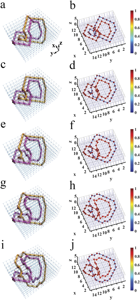
Figure 16. Constructions of five structures between the first structure (figure 4(a)) and the second structure (figure 4(d)) in the continuous change process. In (a), (c), (e), (g) and (i), red (blue) cylinders represent the coupling strengths t = 0.01 (s = 1) in the lattices. Only some sites coupled to neighboring sites by strength ti,j = 0.01 are changed and these sites are nearest neighboring to each other at any two adjacent steps. Red spheres denote the sites occupied by localized eigenstates. We connect these sites in purple and orange tubes. In (b), (d), (f), (h) and (j), we provide the simulated distributions of impedance for electric realizations of (a), (c), (e), (g) and (i), respectively. The value of impedances at each node have been normalized to the maximum impedance.
Download figure:
Standard image High-resolution imageRed (blue) cylinders in the lattices represent the coupling strengths ti,j = 0.01 (sk,l = 1). Red spheres in the lattices represent the sites occupied by localized eigenstates. As shown in figures 16(a), (c), (e), (g) and (i), these sites are exactly those presented in table 14. To illustrate the distribution clearly, we use the purple and orange tubes in figure 16 to connect these sites. We find that they comprise the five structures. So we realize 'discrete' versions of these five structures. The corresponding electric realizations are similar to those above. We connect every two nodes in the electric circuit through the electric capacitors. The nodes with the coordinates presented in table 14 are connected by the small capacitor C1 = 100 pF, and other nodes are connected by the large capacitor C2 = 10 nF. The distributions of large impedances are consistent with those of localized eigenstates in figures 16(b), (d), (f), (h) and (j). We can find that the nodes having large impedances in the circuits are consistent with those sites occupied by localized eigenstates in the lattices.
We also provide the continuous change between the structure in figure 4(d) and the structure in figure 4(f). To realize such continuous change, we need to construct another five structures. The coordinates in table 15 connect with the six adjacent sites through the coupling strength ti,j = 0.01, and the coupling strengths between other sites are sk,l = 1.
Table 15. The coordinates  connect with all adjacent sites through ti,j
= 0.01.
connect with all adjacent sites through ti,j
= 0.01.
| The structure in figure 17(a) | |||||||||
| (2,6,2) | (2,7,1) | (2,8,2) | (2,9,1) | (2,10,2) | (3,11,2) | (4,11,1) | (5,11,2) | (6,11,1) | (7,11,2) |
| (7,12,3) | (8,12,4) | (9,11,4) | (10,11,3) | (11,10,3) | (11,9,4) | (12,8,4) | (12,7,5) | (12,6,4) | (11,5,4) |
| (10,4,4) | (9,3,4) | (8,2,4) | (7,2,3) | (6,2,2) | (5,3,2) | (4,4,2) | (3,5,2) | (4,6,2) | (4,7,1) |
| (4,8,2) | (4,9,1) | (5,9,2) | (6,9,1) | (7,9,2) | (8,9,1) | (9,10,1) | (10,11,1) | (10,12,2) | (9,13,2) |
| (8,14,2) | (7,14,3) | (6,14,4) | (5,13,4) | (4,12,4) | (5,11,4) | (6,10,4) | (7,10,5) | (8,10,4) | (9,9,4) |
| (9,8,5) | (10,7,5) | (10,6,4) | (9,5,4) | (8,4,4) | (7,4,3) | (6,4,2) | (5,5,2) | ||
| The structure in figure 17(c) | |||||||||
| (2,6,2) | (2,7,1) | (2,8,2) | (2,9,1) | (2,10,2) | (3,11,2) | (4,11,1) | (5,11,2) | (6,11,1) | (7,11,2) |
| (7,12,3) | (8,12,4) | (9,11,4) | (10,11,3) | (11,10,3) | (12,9,3) | (12,8,4) | (12,7,5) | (12,6,4) | (11,5,4) |
| (10,4,4) | (9,3,4) | (8,2,4) | (7,2,3) | (6,2,2) | (5,3,2) | (4,4,2) | (3,5,2) | (4,6,2) | (4,7,1) |
| (4,8,2) | (4,9,1) | (5,9,2) | (6,9,1) | (7,9,2) | (8,9,1) | (9,10,1) | (10,11,1) | (10,12,2) | (9,13,2) |
| (8,14,2) | (7,14,3) | (6,14,4) | (6,13,5) | (5,12,5) | (6,11,5) | (7,10,5) | (8,10,4) | (9,10,5) | (10,9,5) |
| (10,8,4) | (10,7,5) | (10,6,4) | (9,5,4) | (8,4,4) | (7,4,3) | (6,4,2) | (5,5,2) | ||
| The structure in figure 17(e) | |||||||||
| (2,6,2) | (2,7,1) | (2,8,2) | (2,9,1) | (2,10,2) | (3,11,2) | (4,11,1) | (5,11,2) | (6,11,1) | (7,11,2) |
| (7,12,3) | (8,12,4) | (9,11,4) | (10,10,4) | (11,10,3) | (12,9,3) | (12,8,4) | (12,7,5) | (12,6,4) | (11,5,4) |
| (10,4,4) | (9,3,4) | (8,2,4) | (7,2,3) | (6,2,2) | (5,3,2) | (4,4,2) | (3,5,2) | (4,6,2) | (4,7,1) |
| (4,8,2) | (4,9,1) | (5,9,2) | (6,9,1) | (7,9,2) | (8,9,1) | (9,10,1) | (10,11,1) | (10,12,2) | (9,13,2) |
| (8,14,2) | (7,14,3) | (7,13,4) | (7,12,5) | (8,11,5) | (9,10,5) | (9,9,4) | (10,8,4) | (10,7,5) | (10,6,4) |
| (9,5,4) | (8,4,4) | (7,4,3) | (6,4,2) | (5,5,2) | |||||
| The structure in figure 17(g) | |||||||||
| (2,6,2) | (2,7,1) | (2,8,2) | (2,9,1) | (2,10,2) | (3,11,2) | (4,11,1) | (5,11,2) | (6,11,1) | (7,11,2) |
| (7,12,3) | (8,12,4) | (9,11,4) | (10,10,4) | (11,10,3) | (12,9,3) | (12,8,4) | (12,7,5) | (12,6,4) | (11,5,4) |
| (10,4,4) | (9,3,4) | (8,2,4) | (7,2,3) | (6,2,2) | (5,3,2) | (4,4,2) | (3,5,2) | (4,6,2) | (4,7,1) |
| (4,8,2) | (4,9,1) | (5,9,2) | (6,9,1) | (7,9,2) | (8,9,1) | (9,10,1) | (10,11,1) | (10,12,2) | (9,13,2) |
| (8,14,2) | (7,14,3) | (8,14,4) | (9,13,4) | (9,12,5) | (10,11,5) | (11,10,5) | (10,9,5) | (10,8,4) | (10,7,5) |
| (10,6,4) | (9,5,4) | (8,4,4) | (7,4,3) | (6,4,2) | (5,5,2) | ||||
| The structure in figure 17(i) | |||||||||
| (2,6,2) | (2,7,1) | (2,8,2) | (2,9,1) | (2,10,2) | (3,11,2) | (4,11,1) | (5,11,2) | (6,11,1) | (7,11,2) |
| (7,12,3) | (8,12,4) | (9,11,4) | (10,10,4) | (11,10,3) | (12,9,3) | (12,8,4) | (12,7,5) | (12,6,4) | (11,5,4) |
| (10,4,4) | (9,3,4) | (8,2,4) | (7,2,3) | (6,2,2) | (5,3,2) | (4,4,2) | (3,5,2) | (4,6,2) | (4,7,1) |
| (4,8,2) | (4,9,1) | (5,9,2) | (6,9,1) | (7,9,2) | (8,9,1) | (9,10,1) | (10,11,1) | (10,12,2) | (9,13,2) |
| (8,14,2) | (9,14,3) | (10,14,4) | (11,13,4) | (11,12,5) | (12,11,5) | (11,10,5) | (10,9,5) | (10,8,4) | (10,7,5) |
| (10,6,4) | (9,5,4) | (8,4,4) | (7,4,3) | (6,4,2) | (5,5,2) |
In figure 17, we provide the realizations of these five structures in the lattices. Red (blue) cylinders in the lattices represent the coupling strengths ti,j = 0.01 (sk,l = 1). Red spheres in the lattices represent the sites occupied by localized eigenstates. As shown in figures 17(a), (c), (e), (g) and (i), these sites are exactly those presented in table 15. To illustrate the distribution clearly, we use the purple and orange tubes in figure 17 to connect these sites. We find that they comprise the five structures. So we realize 'discrete' versions of these five structures. The corresponding electric realizations are similar to those above. We connect every two nodes in the electric circuit through the electric capacitors. The nodes with the coordinates presented in table 15 are connected by the small electric capacitor C1 = 100 pF, and other nodes are connected by the large electric capacitor C2 = 10 nF. The distributions of large impedances are consistent with those of localized eigenstates in figures 17(b), (d), (f), (h) and (j). We can find that the nodes having large impedances in the circuits are consistent with those sites occupied by localized eigenstates in the lattices.
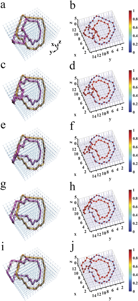
Figure 17. Constructions of five structures between the second structure (figure 4(d)) and the third structure (figure 4(g)) in the continuous change process. In (a), (c), (e), (g) and (i), red (blue) cylinders represent the coupling strengths t = 0.01 (s = 1) in the lattices. Red spheres denote the sites occupied by localized eigenstates. We connect these sites in purple and orange tubes. In (b), (d), (f), (h) and (j), we provide the simulated distributions of impedance for electric realizations of (a), (c), (e), (g) and (i), respectively. The value of impedance at each node has been normalized to the maximum impedance.
Download figure:
Standard image High-resolution image