


Abstract
The ages of the oldest stars shed light on the birth, chemical enrichment, and chemical evolution of the universe. Nucleocosmochronometry provides an avenue to determining the ages of these stars independent from stellar-evolution models. The uranium abundance, which can be determined for metal-poor r-process enhanced (RPE) stars, has been known to constitute one of the most robust chronometers known. So far, U abundance determination has used a single U ii line at
Export citation and abstract BibTeX RIS
1. Introduction
The ages of the oldest stars aid in our understanding of chemical enrichment and evolution in the early universe, the assembly history of our Galaxy (e.g., Marín-Franch et al. 2009; Bonaca et al. 2020; Buder et al. 2022; Rix et al. 2022; Xiang & Rix 2022), and the age of the universe (e.g., Bond et al. 2013; VandenBerg et al. 2014; Jimenez et al. 2019; Valcin et al. 2020; Abdalla et al. 2022). Most techniques used to infer stellar ages, including isochrone-placement and asteroseismology, depend on a detailed understanding of low-metallicity stellar-evolution models, which is challenging and still evolving (e.g., Miglio et al. 2013; Epstein et al. 2014; Joyce & Chaboyer 2015; Tayar et al. 2017; Catelan 2018; Valentini et al. 2019). On the other hand, nucleocosmochronometry, a radioactive-dating technique, offers an independent avenue to determining the ages of some of the oldest stars (Soderblom 2010; Catelan 2018).
Nucleocosmochronometry uses the decay of long-lived actinides, uranium (238U;
One of the major systematic uncertainties in nucleocosmochronometry is the PRs of Th and U to lighter r-process elements like Eu (Goriely & Arnould 2001; Schatz et al. 2002). This issue has been prominently highlighted by the negative Th/Eu stellar ages obtained for 30% of RPE stars, termed as actinide-boost stars (Roederer et al. 2009; Mashonkina et al. 2014; Holmbeck et al. 2018). The negative stellar ages are a result of the observed Th/Eu abundance ratios being higher than the Th/Eu PRs predicted by current r-process models. More generally, the application of the Th/Eu chronometer to RPE stars has led to a large range in ages from 21 to −9 Gyr, even though these stars are metal poor (Holmbeck et al. 2018; Ji & Frebel 2018). These anomalies have indicated that the astrophysical conditions of r-process nucleosynthetic events may be varying event to event, with the PRs of actinides to lighter r-process elements sensitive to these changes. Consequently, no one set of Th/X and U/X PR may be applicable to all RPE stars (Holmbeck et al. 2019a).
On the other hand, the U/Th chronometer results in high-fidelity stellar-age estimates even for the actinide-boost stars (Cayrel et al. 2001; Hill et al. 2002; Frebel et al. 2007; Placco et al. 2017; Holmbeck et al. 2018). Since U and Th have similar nuclear masses and are synthesized along similar reaction channels during the r-process, their PR is robust to major shortcomings of r-process models (Arnould & Takahashi 1999; Goriely & Clerbaux 1999; Schatz et al. 2002). Additionally, any variations in the r-process astrophysical conditions are expected to impact the actinides, U and Th, equally, so that their PR is generally constant across all r-process nucleosynethetic events (e.g., Holmbeck et al. 2019a), with the uncertainty in the predicted value of the PR largely due to the unknown nuclear data of the neutron-rich actinides (Holmbeck et al. 2019b; Lund et al. 2023).
However, it is particularly challenging to reliably determine U abundance. So far, in the context of nucleocosmochronometry, U abundance has been confidently determined for only five highly RPE ([Eu/Fe] > +0.7) stars: namely, CS 31082–001 (Cayrel et al. 2001; Hill et al. 2002), HE 1523–0901 (Frebel et al. 2007), 2MASS J09544277+5246414 (Holmbeck et al. 2018), RAVE J203843.2–002333 (Placco et al. 2017), and CS 29497–004 (Hill et al. 2017). Canonically, and also in the case of these five stars, a single U ii line at
In this study, we have homogeneously determined the U abundance of four highly RPE stars using two novel U ii lines at
Hereafter, this paper is organized as follows: Section 2 describes the observations and data reduction of the stars. Section 3 discusses their atmospheric stellar-parameter estimates. The chemical-abundance analysis of the pertinent elements, including U, Th, and Eu, is described in Section 4. In Section 5, we present the nucleocosmochronometric ages of the stars using the newly derived U, Th, and Eu abundances. Finally, in Section 6, we discuss our results, and in Section 7, we present the main conclusions of this work.
2. Data Acquisition and Reduction
A robust abundance analysis of U requires high signal-to-noise ratio (S/N) and high-resolution spectral data, since U ii transition lines are weak and surrounded by blends. We obtained new spectroscopic data for J0954+5246 and J2038–0023 using the high-resolution spectrographs Keck/HIRES and Magellan/MIKE, respectively. For HE 1523–0901 and CS 31082–001, we utilized Very Large Telescope (VLT)/UVES archival data.
Following the data reduction and radial-velocity correction, the orders of each exposure were normalized using a natural cubic spline function with sigma clipping and the strong lines masked. The normalized orders were coadded and then stitched 15 to furnish the final spectrum of each star. We summarize the spectral data properties of all of the stars in Table 1, including the wavelength range, resolving power, and S/N per pixel of the final spectra.
Table 1. Spectral Data Properties
| Star Name | Telescope/ | Wavelength | Slit | Resolving Power | Total | S/N pix−1 |
|---|---|---|---|---|---|---|
| Instrument | Range (Å) | Width | ( | Exposure (hr) | at 4050 Å | |
| 2MASS J09544277+5246414 | Keck/HIRESb | 3600–6800 | 0 40 40 | 86,600 | 6.6 | 200 |
| RAVE J203843.2–002333 | Magellan/MIKE | 3200–9900 | 035 | 83,000 | 15.6 | 175 |
| HE 1523–0901 | VLT/UVES | 3758–4990 | 045 | 75,000 | 3.0 | 200 |
| CS 31082–001 | VLT/UVES | 3800–5100 | 045 | 70,000 | 2.0 | 125 |
Download table as: ASCIITypeset image
2.1. 2MASS J09544277+5246414
We observed J0954+5246 with Keck/HIRESr (Vogt et al. 1994) on 2021 March 26 for a total of 6.6 hr. The observations were broken down as eight exposures of 1800 s, 1 exposure of 1400 s, and 1 exposure of 1350 s. The observations were taken with the red cross-disperser, using the 5.0 × 040 slit and with 1 × 1 binning, which yielded a resolving power of R ∼ 86,600. We used the blue and the green CCD chip data, which we reduced with MAKEE
16
using standard settings. The full wavelength range of the spectra was 3600–6800 Å. We corrected each spectrum for radial velocity by cross-correlating against a high-resolution spectrum of HD 122563. We normalized, coadded, and stitched the spectra to furnish the final spectrum with S/N per pixel of 185 at 4050 Å.
2.2. RAVE J203843.2–002333
We observed J2038–0023 with Magellan/MIKE (Bernstein et al. 2003) on 2018 July 8, 2018 July 24, 2018 September 26, and 2018 November 11, for a total of 15.6 hr. We used the 035 slit and 2 × 1 binning, which yielded a resolving power of R ∼ 83,000. Data for this star already existed (Placco et al. 2017), but with 2 × 2 binning, which could have undersampled the profiles of the U ii lines, so we reobserved the star. We reduced the spectra from each night, together, using CarPy (Kelson et al. 2000; Kelson 2003) and corrected the radial velocity by cross-correlating against a high-resolution spectrum of HD 122563. We normalized, coadded, and stitched the spectra to furnish the final spectrum with S/N per pixel of 175 at 4050 Å.
2.3. HE 1523–0901
We used the data from Frebel et al. (2007), who observed the star with VLT/UVES (Dekker et al. 2000) in 2005 and 2006, using image slicer No. 2 and 045 slit width to achieve a resolving power of R ∼ 75,000. The data are publicly available on the ESO raw data archive.
17
We used the BLUE 437 nm setting observations from 2006 April 22, 2006 April 23, and 2006 May 19, which amounted to a total exposure time of 3.0 hr. The wavelength range of the final spectrum was 3758–4990 Å, which included all of the lines of interest. We reduced the data using ESOReflex (Freudling et al. 2013), with order extraction set to the recommended linear method for data collected with an image slicer. We corrected the radial velocity of each exposure by cross-correlating with a high-quality rest-frame MIKE/Magellan spectrum of HE 1523–0901. We normalized, coadded, and stitched the spectra to furnish the final spectrum with S/N per pixel of 200 at 4050 Å.
2.4. CS 31082–001
We used data from Hill et al. (2002), who observed the star with VLT/UVES (Dekker et al. 2000) in 2000 using 045 slit width. The data are publicly available on the ESO raw data archive. We used the BLUE arm 380–510 nm setting observations from 2000 October 17 and 2000 October 19, which totaled 2 hr of exposure. The resulting resolving power was R ∼ 75,000. We reduced the data using ESOReflex (Freudling et al. 2013), with order extraction set to the recommended optimal method. We corrected the radial velocity of each exposure by cross-correlating to a high-quality MIKE/Magellan spectrum of HE 1523–0901. We normalized, coadded, and stitched the spectra to furnish the final spectrum with S/N of 125 per pixel at 4050 Å.
3. Stellar Parameters
We derived the stellar parameters of all of the stars spectroscopically. For this purpose, we used SMHr, 18 the next generation spectroscopic analysis software of SMH (Casey 2014). SMHr wraps the radiative transfer code, MOOG (Sneden 1973), and allows for the employment of various grid model atmospheres. We used MOOG with the proper treatment of scattering included 19 (Sobeck et al. 2011) and employed the ATLAS9 grid of 1D plane-parallel model atmospheres computed under the assumption of local thermodynamic equilibrium (Castelli & Kurucz 2003).
We used equivalent widths (EWs) of Fe i and Fe ii lines for stellar parameter determination of all of the stars. We measured the EWs within SMHr by fitting Gaussian or Voigt profiles. We obtained the effective temperature (Teff) by inducing equilibrium in the Fe i line abundances with respect to the excitation potential of the lines, the surface gravity ( ) by minimizing the difference between the mean Fe i and Fe ii abundances, and the microturbulent velocity (
 , and
, and  and
and
Table 2. Stellar Parameters
| Star | Source | Teff |

| [Fe/H] |
|
|---|---|---|---|---|---|
| (K) | (cgs) | (km s−1) | |||
| J0954+5246 | This work | 4410 ± 150 | 0.61 ± 0.30 | −2.96 ± 0.14 | 2.74 ± 0.20 |
| Holmbeck et al. (2018) | 4340 ± 125 | 0.41 ± 0.20 | −2.99 ± 0.10 | 2.28 ± 0.20 | |
| J2038–0023 | This work | 4519 ± 150 | 0.57 ± 0.30 | −3.12 ± 0.12 | 2.26 ± 0.20 |
| Placco et al. (2017) | 4630 ± 100 | 1.20 ± 0.20 | −2.91 ± 0.10 | 2.15 ± 0.20 | |
| HE 1523–0901 | This work | 4607 ± 150 | 0.94 ± 0.30 | −2.98 ± 0.14 | 2.65 ± 0.20 |
| Frebel et al. (2007) | 4630 ± 40 | 1.00 ± 0.30 | −2.95 ± 0.2 | 2.60 ± 0.30 | |
| CS 31082–001 | This work | 4793 ± 150 | 1.36 ± 0.30 | −2.94 ± 0.11 | 1.68 ± 0.20 |
| Hill et al. (2002) | 4825 ± 120 | 1.50 ± 0.30 | −2.9 ± 0.13 | 1.80 ± 0.20 |
Download table as: ASCIITypeset image
The stellar parameters derived in this work agree with those determined previously in the literature within uncertainties for all of the stars in our sample, except for J2038–0023. The primary disagreement for J2038–0023 is in  , where we derived
  = 0.57, whereas Placco et al. (2017) derived
  = 1.20 using the EW technique. Upon further investigation into this discrepancy, we suspect that it mostly originates from different implementations of scattering in MOOG. For homogeneity with the other stars in our sample, we adopt our derived stellar parameters for J2038–0023.
4. Chemical-abundance Analysis
We derived chemical abundances for all of the stars using EWs and spectral synthesis in SMHr. Though abundances for these stars have been previously reported in the literature, we rederived abundances of the relevant elements for a homogeneous and consistent analysis. This enabled us to robustly constrain the transitions directly blended with the U ii lines, as well as those neighboring the U ii lines, which could affect the local continuum placement. We derived abundances of most light elements, including Na, Mg, Al, Si, Ca, Ti, Cr, Fe, and Zn, using the EW method. We derived abundances of the remaining light elements and the neutron-capture (n-cap) elements, including C, N, V, Mn, Sr, Y, Zr, Ba, La, Ce, Pr, Nd, Sm, Eu, Gd, Dy, Tm, Er, Th, and U, with spectral synthesis of ±5 Å regions around the transition lines. For the abundance determination of the light and n-cap elements, we used a subset of the transition list compiled by Roederer et al. (2018). For abundance analysis with spectral synthesis, we generated the atomic-parameters linelists with linemake
20
(Placco et al. 2021), which included the transition wavelengths ( ), and hyperfine structure of the transition lines. We used the updated atomic parameters of CH transitions from Masseron et al. (2014)
21
and r-process isotopic ratios from Sneden et al. (2008) for the spectral synthesis of Ba, Eu, Nd, Sm, Yb, and Pb. We further detail the abundance determination of the U ii line blends, U, Th, and Eu in Sections 4.1–4.4, respectively. We describe uncertainty analysis of the derived abundances in Section 4.5.
), and hyperfine structure of the transition lines. We used the updated atomic parameters of CH transitions from Masseron et al. (2014)
21
and r-process isotopic ratios from Sneden et al. (2008) for the spectral synthesis of Ba, Eu, Nd, Sm, Yb, and Pb. We further detail the abundance determination of the U ii line blends, U, Th, and Eu in Sections 4.1–4.4, respectively. We describe uncertainty analysis of the derived abundances in Section 4.5.
4.1. Blends: Fe, C, N, and La
We took special care to constrain the abundances of elements that have transitions blended with the weak U ii lines. We identified that transitions of Fe i, CH, CN, and La ii are blended with the U ii lines investigated in this work. We obtained the Fe abundance using EW measurements of a subset of acceptable Fe i lines listed in Roederer et al. (2018), for each sample star. We estimated the uncertainty on the mean Fe abundance as the standard deviation in the abundances of the chosen Fe i lines. We determined the C abundance by fitting the
Table 3. Abundances and Isotopic Ratios of U ii Line Blends
| Source | J0954+5246 a | J2038–0023 b | HE 1523–0901 c | CS 31082–001 d | |
|---|---|---|---|---|---|
 (Fe) (Fe) | This Work | 4.55 ± 0.15 | 4.41 ± 0.12 | 4.53 ± 0.14 | 4.58 ± 0.11 |
| Other | 4.51 ± 0.12 | 4.59 ± 0.12 | 4.50 ± 0.20 | 4.60 ± 0.13 | |
 (C) (C) | This Work | 4.97 ± 0.20 | 5.11 ± 0.20 | 5.17 ± 0.20 | 5.75 ± 0.20 |
| Other | 4.94 ± 0.20 | 5.08 ± 0.20 | 5.14 | 5.82 ± 0.05 | |
| 12C/13C | This Work | 4.0 | 4.6 | 3.5 | 19.0 |
| Other | ⋯ | ⋯ | ∼3–4 | >20.0 | |
 (N) (N) | This Work | 5.82 ± 0.20 | 5.56 ± 0.20 | 5.88 ± 0.20 | ⋯ |
| Other | ⋯ | ⋯ | 5.43 | <5.22 | |
 (La) (La) | This Work | −1.06 ± 0.09 | −1.06 ± 0.05 | −0.47 ± 0.11 | −0.65 ± 0.07 |
| Other | −1.15 ± 0.10 | −0.76 ± 0.07 | −0.63 | −0.60 ± 0.04 |
Notes. Source of other work:
a Holmbeck et al. (2018). b Placco et al. (2017). c Frebel et al. (2007). d Hill et al. (2002).Download table as: ASCIITypeset image
4.2. Uranium
So far in the literature, U abundances of RPE stars have been primarily determined using a single U ii line at
In this study, we performed, for the first time, a homogeneous analysis to determine U abundances of four highly RPE stars using three U ii lines at  measurements of the U ii lines from Nilsson et al. (2002a), who measured them with high accuracy by combining their branching fraction calculations with the radiative lifetime measurements of six U ii levels from Lundberg et al. (2001). We list the atomic parameters employed for the three U ii transitions in Table 4.
Table 4. Atomic Parameters of U ii Transition Lines
| Species |
|
|

| % Uncertainty |
|---|---|---|---|---|
| in gf | ||||
| U ii | 3859.57 | 0.036 | −0.067 | 12 |
| U ii | 4050.04 | 0.000 | −0.706 | 7 |
| U ii | 4090.13 | 0.217 | −0.184 | 13 |
Note.
 values and percent uncertainty on gf values taken from Table 2 of Nilsson et al. (2002a). Excitation potential taken from linemake.
Download table as: ASCIITypeset image
We determined the final U abundance of each star as the weighted-average of the U abundances from the three U ii lines, i.e.,  (U) =
(U) =  , where
  is the U abundance from line i and
  for line i (McWilliam et al. 1995; Ji et al. 2019). We detail the method we used to estimate
  , in Section 4.5. For the total uncertainty on the average-weighted U abundances, we accounted for systematic uncertainties (from stellar parameters and blends) and statistical uncertainties (from
  measurement and continuum placement). We discuss this further in Section 4.5. We list the final weighted-average U abundance with the associated total uncertainty for all of the sample stars in Table 5.
Table 5. U, Th, and Eu Abundances and Nucleocosmochronometric Ages a
| Source |
 (X) (X) | J0954+5246 b | J2038–0023 c | HE 1523–0901 d | CS 31082–001 e |
|---|---|---|---|---|---|
| Other Work |
 (U)3859 (U)3859
| −2.13 ± 0.20 | −2.14 ± 0.20 | −2.06 ± 0.12 | −1.92 ± 0.17 |
| This Work |
 (U)3859 (U)3859
| −2.45 ± 0.30 | −2.50 ± 0.26 | −1.93 ± 0.18 | −2.00 ± 0.22 |
 (U)4050 (U)4050
| −2.50 ± 0.33 | −2.34 ± 0.30 | −2.00 ± 0.48 | −1.60 ± 0.21 | |
 (U)4090 (U)4090
| −2.60 ± 0.30 | −2.50 ± 0.24 | −2.15 ± 0.28 | −2.00 ± 0.25 | |
 (U) (U) | −2.50 ± 0.29 | −2.47 ± 0.21 | −1.96 ± 0.25 | −1.87 ± 0.19 | |
| Other Work |
 (Th) (Th) | −1.13 ± 0.10 | −1.24 ± 0.10 | −1.2 ± 0.05 | −0.98 ± 0.13 |
| This Work |
 (Th)4019 (Th)4019
| −1.92 ± 0.09 | − 1.70 ± 0.05 | −1.22 ± 0.11 | −1.18 ± 0.04 |
 (Th)4086 (Th)4086
| −1.70 ± 0.09 | − 1.63 ± 0.05 | −0.95 ± 0.11 | −1.09 ± 0.04 | |
 (Th)4095 (Th)4095
| −1.76 ± 0.09 | − 1.57 ± 0.05 | −1.01 ± 0.11 | −1.10 ± 0.04 | |
 (Th) (Th) | −1.79 ± 0.18 | −1.63 ± 0.21 | −1.06 ± 0.19 | −1.12 ± 0.16 | |
| Other Work |
 (Eu) (Eu) | −1.19 ± 0.10 | −0.75 ± 0.10 | −0.62 ± 0.05 | −0.76 ± 0.13 |
| This Work |
 (Eu) (Eu) | −1.16 ± 0.12 | −1.16 ± 0.13 | −0.53 ± 0.08 | −0.81 ± 0.12 |
| Chronometer | J0954+5246 | J2038–0023 | HE 1523–0901 | CS 31082–001 | |
| Age (Gyr) | U/Th | 11.1 ± 6.4 | 13.5 ± 4.8 | 16.6 ± 5.1 | 11.1 ± 4.0 |
| (±sys ± stat ± PR) | (±5.7 ± 1.9 ± 2.2) | (±3.8 ± 2.1 ± 2.2) | (±4.2 ± 2.0 ± 2.2) | (±2.8 ± 1.8 ± 2.2) | |
| Age (Gyr) | U/Eu | 12.0 ± 4.3 | 11.3 ± 3.1 | 14.2 ± 3.8 | 7.3 ± 2.6 |
| (±sys ± stat ± PR) | (±3.9 ± 1.0 ± 1.6) | (±2.2 ± 1.4 ± 1.6) | (±3.3 ± 1.0 ± 1.6) | (±1.6 ± 1.3 ± 1.6) | |
Notes.
a Nucleocosmochronometric ages listed are obtained in this work. See the text for details on uncertainty estimation for the elemental abundances and stellar ages. b Source of other work: Holmbeck et al. (2018). c Source of other work: Placco et al. (2017). d Source of other work: Frebel et al. (2007). e Source of other work: Hill et al. (2002).Download table as: ASCIITypeset image
4.2.1. The λ 3859 Å U ii Line
While the
To fit the wings of the strong Fe i line, we used the Unsöld approximation (Unsold 1955) multiplied by a factor of −8.77 for the Van der Waals hydrogen collision-damping coefficient of the Fe i line, for all of the sample stars. Furthermore, we adjusted the derived Fe i abundances of the stars by −0.15, −0.05, +0.02, and +0.03 dex for J0954+5246, J2038–0023, HE 1523–0901, and CS 31082–001, respectively. For most of the stars, the adjustment made to the derived Fe i abundance of the star is small and lies within the uncertainty on the Fe i abundance.
To fit the CN feature, we adjusted the derived N abundance of the stars by +0.0, +0.04, and +0.12 dex for J0954+5246, J2038–0023, and HE 1523–0901, respectively. We find these adjustments acceptable, since they are within the ±0.2 dex uncertainty on the derived N abundances. For CS 31082–001, we used  (N) = 5.22, which is the upper limit placed on the N abundance by Hill et al. (2002), as we could not derive a reliable N abundance for the star. We used the derived C abundance of the stars without any adjustments.
For the purpose of a better fit to the neighboring line features, we blueshifted the transition wavelength of the Nd ii line at 3859.42 Å and the Fe i line at 3859.21 Å by 0.07 Å. To fit the Nd ii line, we adjusted the derived Nd ii abundance of the stars by −0.12, +0.0, +0.04, and −0.05 dex for J0954+5246, J2038–0023, HE 1523–0901, and CS 31082–001, respectively. The adjustment is small for most stars and within the uncertainty of the Nd abundance.
We determined  (U)3859 = −2.45, −2.50, −1.93, and −2.0 for J0954+5246, J2038–0023, HE 1523–0901, and CS 31082–001, respectively. In Figure 1, we show the resulting best-fit spectral synthesis model for the observed data of each star, along with the residuals between the model and the data. We also depict the ±0.2 dex abundance variation from the derived
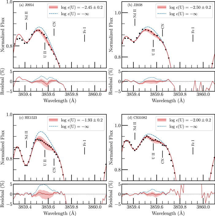
Figure 1. Spectral synthesis of the U ii line at
Download figure:
Standard image High-resolution image4.2.2. The 4050 Å U ii
The  = 0.11 for the La ii line from Corliss & Bozman (1962), but we used an updated
  = 0.428, as measured by Bord et al. (1996). We substantiated this choice with spectral synthesis of the La ii line in RPE stars with minimal U contamination, which showed that the Bord et al. (1996) value provides a better fit to the observed spectra of these stars. Additionally, we blueshifted the transition wavelength of the La ii line by 0.02 Å to enable a better fit to the observed data. We also account for the hyperfine splitting (HFS) structure of this La ii line, as described in the Appendix. We applied the described prescription for the La ii line uniformly across all of the sample stars to determine their U abundances. We employed the derived La abundance of each star in the spectral synthesis without any adjustment.
We determined  (U)4050 = −2.50, −2.34, −2.00, and −1.60 for J0954+5246, J2038–0023, HE 1523–0901, and CS 31082–001, respectively. We show the corresponding best-fit spectral synthesis models for all of the stars in Figure 2, along with the resulting residuals between the model and the observed data. We also depict ±0.2 dex variations in the
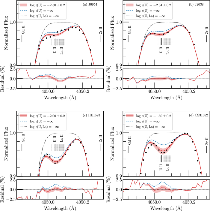
Figure 2. Spectral synthesis of the U ii line at
Download figure:
Standard image High-resolution image4.2.3. The λ 4090 Å U ii Line
The  (U)4090 = −2.60, −2.50, −2.15, and −2.00 for J0954+5246, J2038–0023, HE 1523–0901, and CS 31082–001, respectively. We show the corresponding best-fit spectral synthesis models for all of the stars in Figure 3, along with residuals between the models and the observed data. We also depict ±0.2 variation in the best-fit
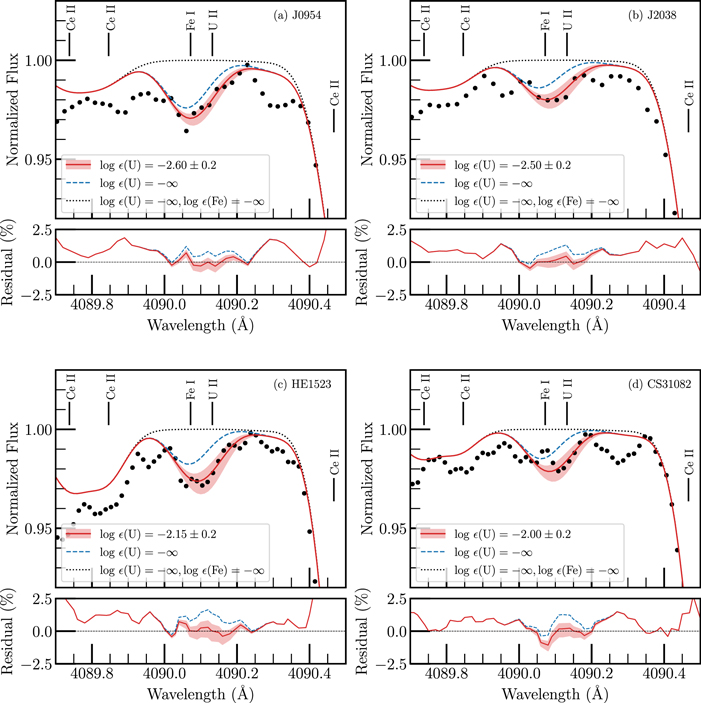
Figure 3. Spectral synthesis of the U ii line at
Download figure:
Standard image High-resolution image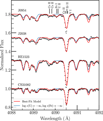
Figure 4. Spectral synthesis around the
Download figure:
Standard image High-resolution image4.3. Thorium
We determined Th abundances for all of the sample stars using Th ii lines at  values from Nilsson et al. (2002b).
The Th ii line at  (Th)4019 = −1.92, −1.70, −1.22, and −1.18 for J0954+5246, J2038–0023, HE 1523–0901, and CS 31082–001, respectively. The corresponding best-fit spectral synthesis model is shown in Figure 5 for each star, along with the residual between the mode and the observed data. We note that the synthetic spectrum is overestimated around the
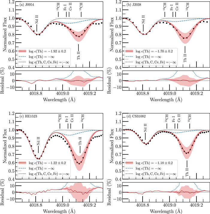
Figure 5. Spectral synthesis of the Th ii line at
Download figure:
Standard image High-resolution imageThe Th ii line at  (Th)4086 = −1.70, −1.63, −0.95, and −1.09 for J0954+5246, J2038–0023, HE 1523–0901, and CS 31082–001. For the spectral synthesis of CS 31082–001, we adjusted the derived Ce abundance of the star by −0.05 dex.
The Th ii line at  (Th)4095 = −1.76, −1.57, −1.01, and −1.10 for J0954+5246, J2038–0023, HE 1523–0901, and CS 31082–001, respectively.
The final Th abundance of each sample star was obtained as the mean of the  (Th) = −1.79, −1.31, −1.06, and −1.12 for J0954+5246, J2038–0023, HE 1523–0901, and CS 31082–001, respectively. We list the Th abundances obtained for each line and the corresponding mean Th abundance for each star in Table 5, along with the uncertainty estimates. Table 5 also lists the Th abundances determined in previous literature studies for comparison. For J0954+5246, HE 1523–0901, and CS 31082–001, we obtain good agreement with the Th abundances published in the literature. For J2038–0023, we note some discrepancy, which we attribute to the difference in the adopted stellar parameters (see Section 3).
4.4. Europium
We determined the Eu abundance of each sample star using Eu ii lines at  (Eu) = −1.16, −1.16, −0.53, and −0.81 for J0954+5246, J2038–0023, HE 1523–0901, and CS 31082–001, respectively. We list the mean Eu abundance, along with the uncertainty estimates and Eu abundance estimates from previous literature studies in Table 5. For J0954+5246, HE 1523–0901, and CS 31082–001, we find our derived Eu abundances to be in good agreement with the literature estimates within uncertainties. For J2038–0023, we note a discrepancy in the abundances, which we attribute to the difference in the adopted stellar parameters.
4.5. Uncertainty Analysis
For the U abundances of the sample stars, we homogeneously accounted for various sources of systematic ( , and
, and  ,
,  values (
 ,
,
Table 6. Abundance Uncertainties
 (cgs) (cgs) | 
| ||||||||
|---|---|---|---|---|---|---|---|---|---|
| J0954+5246 | +150 | +0.30 | +0.20 | ±1 | ±0.5% | ||||
 (U)3859 (U)3859
| +0.10 | +0.10 | +0.05 | ±0.23 | ±0.27 | ±0.05 | ±0.10 | ±0.11 | ±0.30 |
 (U)4050 (U)4050
| +0.05 | +0.05 | +0.02 | ±0.30 | ±0.31 | ±0.03 | ±0.10 | ±0.10 | ±0.33 |
 (U)4090 (U)4090
| +0.08 | +0.09 | +0.04 | ±0.23 | ±0.26 | ±0.06 | ±0.15 | ±0.15 | ±0.30 |
 (U) (U) | +0.08 | +0.08 | +0.04 | ±0.25 | ±0.28 | ⋯ | ⋯ | ±0.07 | ±0.29 |
 (Th) (Th) | +0.15 | +0.08 | +0.00 | ⋯ | ±0.17 | ⋯ | ⋯ | ±0.05 | ±0.18 |
 (Eu) (Eu) | +0.09 | +0.07 | −0.02 | ⋯ | ±0.12 | ⋯ | ⋯ | ±0.01 | ±0.12 |
 (U/Th) (U/Th) | −0.07 | +0.00 | −0.00 | ±0.25 | ±0.26 | ⋯ | ⋯ | ±0.09 | ±0.28 |
 (U/Eu) (U/Eu) | −0.01 | +0.01 | +0.06 | ±0.25 | ±0.26 | ⋯ | ⋯ | ±0.07 | ±0.27 |
| J2038–0023 | +150 | +0.30 | +0.20 | ±1 | ±0.5% | ||||
 (U)3859 (U)3859
| +0.10 | +0.05 | +0.00 | ±0.20 | ±0.23 | ±0.06 | ±0.10 | ±0.12 | ±0.26 |
 (U)4050 (U)4050
| +0.04 | +0.17 | +0.04 | ±0.14 | ±0.23 | ±0.04 | ±0.20 | ±0.20 | ±0.31 |
 (U)4090 (U)4090
| +0.10 | +0.08 | +0.02 | ±0.08 | ±0.15 | ±0.05 | ±0.20 | ±0.21 | ±0.26 |
 (U) (U) | +0.08 | +0.10 | +0.02 | ±0.14 | ±0.19 | ⋯ | ⋯ | ±0.09 | ±0.21 |
 (Th) (Th) | +0.18 | +0.11 | +0.01 | ⋯ | ±0.21 | ⋯ | ⋯ | ±0.03 | ±0.21 |
 (Eu) (Eu) | +0.11 | +0.07 | +0.00 | ⋯ | ±0.13 | ⋯ | ⋯ | ±0.02 | ±0.13 |
 (U/Th) (U/Th) | −0.10 | −0.01 | +0.01 | ±0.14 | ±0.17 | ⋯ | ⋯ | ±0.10 | ±0.20 |
 (U/Eu) (U/Eu) | −0.03 | +0.03 | +0.02 | ±0.14 | ±0.15 | ⋯ | ⋯ | ±0.09 | ±0.17 |
| HE 1523–0901 | +150 | +0.30 | +0.20 | ±1 | ±0.5% | ||||
 (U)3859 (U)3859
| +0.10 | +0.10 | +0.03 | ±0.08 | ±0.17 | ±0.04 | ±0.06 | ±0.07 | ±0.18 |
 (U)4050 (U)4050
| +0.01 | +0.25 | +0.20 | ±0.25 | ±0.41 | ±0.03 | ±0.25 | ±0.25 | ±0.48 |
 (U)4090 (U)4090
| +0.10 | +0.10 | +0.05 | ±0.11 | ±0.19 | ±0.05 | ±0.21 | ±0.22 | ±0.28 |
 (U) (U) | +0.07 | +0.15 | +0.09 | ±0.15 | ±0.24 | ⋯ | ⋯ | ±0.07 | ±0.25 |
 (Th) (Th) | +0.14 | +0.11 | +0.0 | ⋯ | ±0.18 | ⋯ | ⋯ | ±0.06 | ±0.19 |
 (Eu) (Eu) | +0.06 | +0.04 | −0.03 | ⋯ | ±0.08 | ⋯ | ⋯ | ±0.02 | ±0.08 |
 (U/Th) (U/Th) | −0.07 | +0.04 | +0.09 | ±0.15 | ±0.19 | ⋯ | ⋯ | ±0.09 | ±0.21 |
 (U/Eu) (U/Eu) | +0.01 | +0.11 | +0.12 | ±0.15 | ±0.22 | ⋯ | ⋯ | ±0.07 | ±0.23 |
| CS 31082–001 | +150 | +0.30 | +0.20 | ±1 | ±0.5% | ||||
 (U)3859 (U)3859
| +0.10 | +0.10 | +0.00 | ±0.13 | ±0.19 | ±0.05 | ±0.10 | ±0.11 | ±0.22 |
 (U)4050 (U)4050
| +0.05 | +0.12 | +0.03 | ±0.10 | ±0.17 | ±0.03 | ±0.13 | ±0.13 | ±0.21 |
 (U)4090 (U)4090
| +0.10 | +0.10 | +0.00 | ±0.07 | ±0.16 | ±0.06 | ±0.18 | ±0.19 | ±0.25 |
 (U) (U) | +0.08 | +0.11 | +0.01 | ±0.10 | ±0.17 | ⋯ | ⋯ | ±0.08 | ±0.19 |
 (Th) (Th) | +0.14 | +0.06 | −0.02 | ⋯ | ±0.15 | ⋯ | ⋯ | ±0.02 | ±0.16 |
 (Eu) (Eu) | +0.07 | +0.08 | −0.01 | ⋯ | ±0.11 | ⋯ | ⋯ | ±0.05 | ±0.12 |
 (U/Th) (U/Th) | −0.06 | +0.05 | +0.03 | ±0.10 | ±0.13 | ⋯ | ⋯ | ±0.08 | ±0.15 |
 (U/Eu) (U/Eu) | +0.01 | +0.03 | +0.02 | ±0.10 | ±0.11 | ⋯ | ⋯ | ±0.09 | ±0.14 |
Download table as: ASCIITypeset image
To estimate U abundance uncertainties from stellar parameters, we independently changed each stellar parameter by its uncertainty. We thus changed Teff by +150 K,  by +0.3 dex, and
  , and
, and
We estimated
We estimated  ) through varying the
  values by the measurement uncertaintues listed in Nilsson et al. (2002a) and rederiving the U abundances. We estimated
We determined the total uncertainty ( ),
),  ) and
) and
For the final U abundance of each sample star, we take the weighted-average of the U abundances from the three U ii lines. Therefore,  (U) =
(U) =  , where
  is the U abundance from line i and
  . Here
  ),
),  ),
),  . We list the final
We also determined systematic and statistical uncertainties for the Th and Eu abundances of all of the stars. We determined  , and
, and
5. Ages with Novel U ii Lines
The U abundance of a star can be used to determine the star's age using nucleocosmochronometry. We homogeneously determined ages for J0954+5246, J2038–0023, HE 1523–0901, and CS 31082–001, for the first time with U abundance derived using three U ii lines. We determined the ages using Equations (1) and (2) for the U/Th and U/Eu chronometers, respectively (Cayrel et al. 2001)


Here  (U/X)0 is the PR of the chronometer and
  (U/X)obs is the present-day abundance ratio of the chronometer as determined from this work. We took PRs from Schatz et al. (2002), who used waiting-point calculations to estimate site-independent PRs of r-process elements. We list the final ages from the two chronometers and the associated uncertainties in Table 5. We find the U/Th and U/Eu ages agreeing for all of the stars within uncertainties. There is a relatively large discrepancy between the U/Th and U/Eu ages of CS 31082–001, which can be attributed to its actinide-boost nature.
We estimated the uncertainty on the ages by propagating the uncertainties of the PRs and the present-day observed abundance ratios. As a result, our age uncertainties consist of statistical, systematic, and PR components. We obtained the uncertainty on the PRs from Schatz et al. (2002), which are 0.10 dex for the U/Th chronometer and 0.11 dex for the U/Eu chronometer. We determined  ,
,
6. Discussion
To test the reliability of the two new U ii lines at
6.1. Reliability of the New U ii Lines: Line Abundances and Uncertainties
Table 5 lists the final U abundance determined at each U ii line, along with its estimated uncertainty, for all of the sample stars. We note that the U abundances from the three U ii lines agree well, within uncertainties, for all of the sample stars. We also find that the
Moreover, we find that in the case for all of the sample stars, the uncertainties on the U abundances of all three U ii lines are of the same order. This indicates that the new U ii lines provide similar precision for U abundance determination as the canonical
We note, however, an exceptionally high uncertainty estimated for the
As noted in Section 4.2, even though the spectral synthesis fits to the U ii lines are good—the goodness of the fits is further corroborated by the agreement between U abundances from the different U ii lines—there is indication of unidentified features in the
6.2. Reliability of the New U ii Lines: Residuals between Line Abundances
We further demonstrate the reliability of the new U ii lines with Figure 6, which shows (i) the residuals between the  , [Fe/H], [C/Fe], [Eu/Fe], and spectrum S/N in different panels. The uncertainties on the residual data points are calculated by propagating the total uncertainties of the individual line abundances.
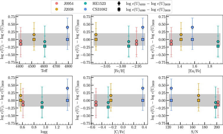
Figure 6. For all of the sample stars, residuals between the  , [Fe/H], [C/Fe], and S/N at 4050 Å of the respective stars in different panels. A gray-shaded region for residuals within ±0.2 dex is also shown.
Download figure:
Standard image High-resolution imageFirst, we note that the residuals of the U abundances are all within ±0.2 dex (shown by the shaded gray region) for all of the stars. For CS 31082–001, while we find that the residual between the
Second, we note that the residuals of the U abundances show no discernible trend with respect to Teff,  , [Fe/H], [C/Fe], [Eu/Fe], and spectrum S/N. This indicates that our current spectral synthesis models are of high fidelity and no identifiable systematic biases are being percolated to the U abundance determinations. Together, the ±0.2 dex range of the residuals between the U ii line abundances and the absence of any significant trend in the residuals with respect to key atmospheric and chemical properties as well as the data quality of the sample stars establish the reliability of the two new U ii new lines at
6.3. Mean U Abundance with Multiple U ii Lines
We provide revised U abundances for the RPE stars, J0954+5246, J2038–0023, HE 1523–0901, and CS 31082–001 via a homogeneous analysis of the three U ii lines at
We compare the final weighted-average U abundances estimated in this work to previous literature estimates of  (see Section 3). Nevertheless, our U/Th and U/Eu nucleocosmochronometric age estimates compare well with those reported in Placco et al. (2017; see Section 5).
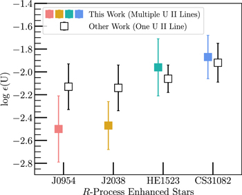
Figure 7. Weighted-average U abundances derived in this work with U ii lines at
Download figure:
Standard image High-resolution imageWe also discuss the uncertainty estimates on the final U abundances as determined in this work compared to previous literature estimates. In the case of J0954+5246 and HE 1523–0901, the total uncertainty estimated for the final weighted-average U abundance in this work is larger than the uncertainty quoted by the respective previous literature studies for their final
6.4. Ages with Mean U Abundances
For every sample star, we determined two stellar ages, one using the U/Th chronometer and another using the U/Eu chronometer. We list the resulting ages in Table 5. There is good agreement between the U/Th and U/Eu ages of J0954+5246, J2038–0023, and HE 1523–0901. For CS 31082–001, the U/Eu age is ∼4.0 Gyr lower than the U/Th age due to its actinide-boost nature (Cayrel et al. 2001; Hill et al. 2002; Schatz et al. 2002). Even then, the U/Th and U/Eu ages of CS 31082–001 agree within uncertainties.
For stellar age uncertainties, we took into account systematic, statistical, and PR uncertainties as described in Section 5. These individual age uncertainty components are listed in Table 5, along with the total age uncertainties. For the U/Th and U/Eu stellar ages of all of the sample stars, the systematic uncertainties are the largest (and also the most dominant, in many cases), followed by the PR uncertainties and then the statistical uncertainties. Specifically, the systematic uncertainties of the stellar ages are driven by the large U abundance uncertainties from the blending elements.
The resulting total uncertainties on the ages of the sample stars are on the order of ∼4-6 Gyr for the U/Th ages and ∼3-4 Gyr for the the U/Eu ages. The U/Eu ages are more precise (although not necessarily more accurate) than the U/Th counterpart because of the shorter half-life of U, relative to Th. We estimate that to achieve a precision of 1 Gyr for the U/Th (U/Eu) ages, the systematic, statistical, and PR uncertainty components will each have to be driven down to less than 0.03 (0.04) dex, which might be challenging given the current limitations of unconstrained atomic data, LTE models, and uncertain r-process PRs. Improvements in these areas are thus highly encouraged.
We note that we have not taken into account the systematic uncertainties associated with using just one set of theoretical PRs (from Schatz et al. 2002). Other r-process models have predicted slightly varying PRs for U/Th and U/Eu (e.g., Goriely & Arnould 2001; Farouqi et al. 2010). However, since the aim of this study was to investigate stellar ages estimated with revised U abundances from multiple U ii lines, we find using one set of PRs sufficient for the analysis.
We compare all of the stellar ages determined in this work to previous literature results in Figure 8, which shows the U/Th and U/Eu ages in the top and bottom panels, respectively. The dashed-black line in Figure 8 indicates the age of the universe, as determined by the Planck mission (Planck Collaboration et al. 2016). For the literature ages of J0954+5246 (Holmbeck et al. 2018), J2038–0023 (Placco et al. 2017), and HE 1523–0901 (Frebel et al. 2007), we display the ages determined by the respective studies using, specifically, the PRs of Schatz et al. (2002) to facilitate a consistent comparison to our age estimates. For CS 31082–001, Hill et al. (2002) determined U/Th age using the PR from Goriely & Arnould (2001), which we display. Also, Hill et al. (2002) did not determine the U/Eu stellar age of the CS 31082–001.
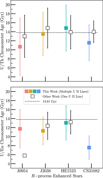
Figure 8. Nucleocosmochronometric ages from this work (colored data points) and previous literature work (white data points) using the U/Th (top panel) and U/Eu (bottom panel) chronometers. The age of the universe is shown as the dashed-black line (Planck Collaboration et al. 2016). For the ages of this work, the weighted-average U, Th, and Eu abundances from multiple transition lines were used. Literature ages were taken from Holmbeck et al. (2018) for J0954+5246, Placco et al. (2017) for RAVE J203843.2–002333, Frebel et al. (2007) for HE 1523–0901, and Hill et al. (2002) for CS 31082–001.
Download figure:
Standard image High-resolution imageWe find that our stellar ages mostly agree well with previous literature results within uncertainties. The exception to this case is the U/Eu age of J0954+5246, which is much higher than previously determined in the literature. We attribute this discrepancy to a lower U abundance determined in this work relative to that determined in Holmbeck et al. (2018; see Section 6.3 more details). We also determined lower Th abundance relative to Holmbeck et al. (2018) so that in the U/Th ratio, the offset in the abundances is canceled.
7. Conclusions
Uranium abundances of metal-poor RPE stars enable stellar age determination independent from stellar-evolution models, using nucleocosmochronometry. U abundances of a large sample of RPE stars may also enable important constraints on the astrophysical conditions and nuclear physics of r-process enrichment events, by probing the production of the actinides. However, U abundance determination has been limited to using a single U ii line at
We test the utility of the
We performed a detailed uncertainty analysis of the U abundances by taking into account systematic uncertainties from stellar parameters and blends, as well as statistical uncertainties from continuum placement and  measurements. We find that all three U ii lines provide similar precision of ∼0.2–0.3 dex. On the other hand, for the weighted-average U abundance, the uncertainties are on the order of ∼0.2 dex. This underscores the advantage of using multiple U ii lines. Moreover, any unconstrained systematic biases associated with a particular U ii line are mitigated in the average abundance from multiple U ii lines.
We also obtained homogeneous ages for the stars with the U/Th and U/Eu chronometers and using the U, Th, and Eu abundances as derived in this work from multiple transition lines of each element. As seen in Figure 8, we find that the newly obtained ages are reasonable and in agreement with previous literature estimates within uncertainties. For the uncertainties on the ages, we estimated the systematic, statistical, and PR uncertainty components for all of the stars. The resulting total uncertainties on the ages of the sample stars are on the order of ∼4–6 Gyr for the U/Th ages and ∼3–4 Gyr for the U/Eu ages.
To improve the uncertainties on the U abundances and subsequently stellar ages, it will be necessary to address systematic uncertainties from the blends and stellar parameters. Additionally, a substantial component of U abundance uncertainties is contributed to fitting uncertainties like continuum placement. As a result, studies of these new U ii-line spectral regions are recommended to better constrain the atomic parameters of the blends and to identify unknown neighboring transitions, which will improve the confidence in the continuum placement.
Another source of uncertainty on the stellar ages is the poorly known nuclear physics that enters into the predicted U/Th and U/Eu PRs. Upcoming studies at facilities such as the N = 126 Factory at Argonne National Laboratory (Savard et al. 2020) and the Facility for Rare Isotope Beams (Castelvecchi 2022) will reach many heavy, neutron-rich species whose properties are crucial for understanding actinide production. These anticipated advances in atomic and nuclear physics will contribute to the overarching goal of improving the precision of nucleocosmochronometry.
Throughout the rest of the decade, we are expecting an influx of new spectroscopic data, specifically for RPE stars, from surveys such as that by the R-Process Alliance (Hansen et al. 2018; Sakari et al. 2018; Ezzeddine et al. 2020; Holmbeck et al. 2020), 4MOST (de Jong et al. 2019), and WEAVE (Dalton et al. 2012). Reliable U abundance determination of RPE stars will be critical in obtaining precise and robust nucleocosmochronometric ages of some of the oldest stars. Precise nucleocosmochronometric ages, combined with chemo-dynamical information, can aid in our understanding of the chemical enrichment and evolution in the early universe, especially of the r-process elements, as well as the assembly history of our galaxy. Additionally, reliable U abundances for a large sample of RPE stars can shed light on the extent of actinide-variation in RPE stars and its origin. To that end, the results of this work open up a new avenue to reliably determine U abundances and nucleocosmochronometric ages for a large sample of RPE stars with multiple U ii lines.
S.P.S. acknowledges Jamie Tayar for useful conversations on stellar ages and other comments. R.E. acknowledges support from NSF grant AST-2206263. A.P.J. was supported by NASA through Hubble Fellowship grant HST-HF2-51393.001 awarded by the Space Telescope Science Institute, which is operated by the Association of Universities for Research in Astronomy, Inc., for NASA, under contract NAS5-26555. A.P.J. also acknowledges support from a Carnegie Fellowship and the Thacher Research Award in Astronomy. T.T.H. acknowledges support from the Swedish Research Council (VR 2021-05556). This project initiated during M.C.'s 2018 sabbatical stay at Carnegie Observatories, and he is very grateful to the faculty and staff there for their hospitality and generous support. Additional support for M.C. is provided by the Ministry for the Economy, Development, and Tourism's Millennium Science Initiative through grant ICN12_12009, awarded to the Millennium Institute of Astrophysics (MAS), and by Proyecto Basal CATA ACE210002 and FB210003. I.U.R. acknowledges support from the U.S. National Science Foundation (NSF) (grants PHY 14-30152—Physics Frontier Center/JINA-CEE, AST 1815403/1815767, and AST 2205847), and the NASA Astrophysics Data Analysis Program, grant 80NSSC21K0627. E.M.H. acknowledges support for this work provided by NASA through the NASA Hubble Fellowship grant HST-HF2-51481.001 awarded by the Space Telescope Science Institute, which is operated by the Association of Universities for Research in Astronomy, Inc., for NASA, under contract NAS5-26555. T.C.B. acknowledges partial support for this work from grant PHY 14-30152; Physics Frontier Center/JINA Center for the Evolution of the Elements (JINA-CEE), awarded by the US National Science Foundation. This work has made use of data from the European Space Agency (ESA) mission Gaia (https://www.cosmos.esa.int/gaia), processed by the Gaia Data Processing and Analysis Consortium (DPAC, https://www.cosmos.esa.int/web/gaia/dpac/consortium). Funding for the DPAC has been provided by national institutions, in particular the institutions participating in the Gaia Multilateral Agreement. The authors wish to recognize and acknowledge the very significant cultural role and reverence that the summit of Maunakea has always had within the indigenous Hawaiian community. We are most fortunate to have the opportunity to conduct observations from this mountain.
Facilities: Keck (HIRES) - , Magellan (MIKE) - , VLT (UVES). -
Software: astropy (Astropy Collaboration et al. 2013), MAKEE (https://sites.astro.caltech.edu/~tb/makee/), CarPy (Kelson et al. 2000; Kelson 2003), ESOReflex (Freudling et al. 2013), MOOG (https://github.com/alexji/moog17scat and Sneden 1973), SMHr (https://github.com/eholmbeck/smhr-rpa/tree/refactor-scatterplot and https://github.com/andycasey/smhr/tree/refactor-scatterplot).
Appendix: Hyperfine Splitting of the La ii
λ 4050 Line
The U ii line at 4050.04 Å is blended with a stronger La ii line at 4050.073 Å. There is one dominant naturally occurring isotope of La, 139La, which has nuclear spin I = 7/2. This nonzero nuclear spin creates HFS structure, which desaturates the line and is thus important to account for in stellar abundance work. We adopt the HFS A and B constants for the upper and lower levels of this transition from the measurements of Furmann et al. (2008a, 2008b). We compute the complete line component pattern for this line following the procedure described in Appendix A1 of Ivans et al. (2006). We calculate the center-of-gravity wavenumber of this line from the energy levels given in the National Institute of Standards and Technology (NIST) Atomic Spectra Database (ASD; Kramida et al. 2021). We convert to the center-of-gravity air wavelength using the standard index of air (Peck & Reeder 1972). Table A1 lists the line component positions relative to these values. The strengths are normalized to sum to 1.0.
Table A1. Hyperfine Structure Line Component Pattern for the La ii
| Wavenumber |
| Fupper | Flower | Component Position | Component Position | Strength |
|---|---|---|---|---|---|---|
| (cm−1) | (Å) | (cm−1) | (Å) | |||
| 24683.94 | 4050.073 | 5.5 | 6.5 | +0.188754 | −0.030979 | 0.25000 |
| 24683.94 | 4050.073 | 5.5 | 5.5 | +0.097552 | −0.016010 | 0.04545 |
| 24683.94 | 4050.073 | 5.5 | 4.5 | +0.018860 | −0.003095 | 0.00455 |
| 24683.94 | 4050.073 | 4.5 | 5.5 | +0.066181 | −0.010862 | 0.16883 |
| 24683.94 | 4050.073 | 4.5 | 4.5 | −0.012510 | +0.002053 | 0.06926 |
| 24683.94 | 4050.073 | 4.5 | 3.5 | −0.077930 | +0.012790 | 0.01190 |
| 24683.94 | 4050.073 | 3.5 | 4.5 | −0.037194 | +0.006104 | 0.10476 |
| 24683.94 | 4050.073 | 3.5 | 3.5 | −0.102614 | +0.016842 | 0.07483 |
| 24683.94 | 4050.073 | 3.5 | 2.5 | −0.154142 | +0.025298 | 0.02041 |
| 24683.94 | 4050.073 | 2.5 | 3.5 | −0.121201 | +0.019892 | 0.05612 |
| 24683.94 | 4050.073 | 2.5 | 2.5 | −0.172729 | +0.028349 | 0.06531 |
| 24683.94 | 4050.073 | 2.5 | 1.5 | −0.209879 | +0.034446 | 0.02857 |
| 24683.94 | 4050.073 | 1.5 | 2.5 | −0.185678 | +0.030474 | 0.02143 |
| 24683.94 | 4050.073 | 1.5 | 1.5 | −0.222828 | +0.036572 | 0.04286 |
| 24683.94 | 4050.073 | 1.5 | 0.5 | −0.245257 | +0.040253 | 0.03571 |
Note. Energy levels from the NIST ASD and the index of air (Peck & Reeder 1972) are used to compute the center-of-gravity wavenumbers and air wavelengths,
Download table as: ASCIITypeset image
Footnotes
- *
Some of the data presented herein were obtained at the W. M. Keck Observatory, which is operated as a scientific partnership among the California Institute of Technology, the University of California, and the National Aeronautics and Space Administration. The Observatory was made possible by the generous financial support of the W. M. Keck Foundation. Additionally, this work is based on observations made with ESO Telescopes at the La Silla Paranal Observatory under program IDs 275.D-5028(A), 077.D-0453(A), and 165.N-0276(A). This paper also includes data gathered with the 6.5 meter Magellan Telescopes located at Las Campanas Observatory, Chile.
- 14
![$[{\rm{A}}/{\rm{B}}]=\mathrm{log}{({N}_{{\rm{A}}}/{N}_{{\rm{B}}})}_{\mathrm{Star}}-\mathrm{log}{({N}_{{\rm{A}}}/{N}_{{\rm{B}}})}_{\mathrm{Solar}}$](data:image/png;base64,iVBORw0KGgoAAAANSUhEUgAAAAEAAAABCAQAAAC1HAwCAAAAC0lEQVR42mNkYAAAAAYAAjCB0C8AAAAASUVORK5CYII=) , where N is the number density of the element.
, where N is the number density of the element. - 15
- 16
- 17
- 18
- 19
- 20
- 21
- 22
An exception to this case is Roederer et al. (2018), who also used the U ii line at
λ 4241 Å to place an upper limit on the U abundance of an RPE star, HD 222925.
![$[{\rm{A}}/{\rm{B}}]=\mathrm{log}{({N}_{{\rm{A}}}/{N}_{{\rm{B}}})}_{\mathrm{Star}}-\mathrm{log}{({N}_{{\rm{A}}}/{N}_{{\rm{B}}})}_{\mathrm{Solar}}$](https://content.cld.iop.org/journals/0004-637X/948/2/122/revision1/apjacb8afieqn1.gif)