

Abstract
Observation of planetary transits and other cutting-edge scientific missions can take advantage of affordable nanosatellites to probe interesting stellar targets. PicSat, a CubeSat dedicated to observing the Beta Pictoris star system, was designed to provide high-precision star pointing, a critical requirement for planetary transit detection. PicSat's Attitude Determination and Control System, responsible for delivering high-accuracy spacecraft pointing, requires dedicated development based on dynamic simulators. This paper presents a dynamic attitude and orbit propagation simulator for CubeSats in low Earth orbit, as well as for its de-tumbling mode. Validation has been performed through PicSat's in-flight data. High-precision dynamic models have been obtained for both attitude and orbit. Such models are well suited to the different mission phases, from spacecraft design to data exploitation. It is, therefore, a crucial tool to minimize the chance of failure of both the platform and the payload, especially in satellites such as PicSat, whose pointing depends on both. PicSat left an enduring legacy: its platform data allow us to obtain flight models that will be valuable for future missions.
Export citation and abstract BibTeX RIS

Original content from this work may be used under the terms of the Creative Commons Attribution 3.0 licence. Any further distribution of this work must maintain attribution to the author(s) and the title of the work, journal citation and DOI.
1. Introduction
PicSat (Nowak et al. 2018) was a 3U (3 unit) CubeSat launched in 2018 and designed to observe the Beta Pictoris star system. The system comprises
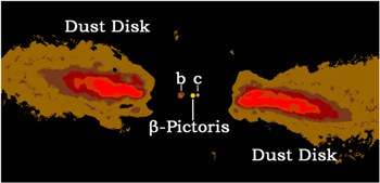
Figure 1. Artistic representation of the Beta Pictoris system by Nicholas W. Beeson based on an image whose credit is: Axel Quetz/MPIA Graphics Department. Licensed under CC BY‒SA 4.0.
Download figure:
Standard image High-resolution imageA CubeSat is a small satellite composed of unit cubes of 10 cm × 10 cm × 10 cm, and no more than 1.33 kg (∼2.9 lb) per unit. The CubeSat concept was first proposed by California Polytechnic State University and Stanford University in 1999 Puig-Suari et al. (2001). A Cubesat often employs commercial off-the-shelf (COTS) components and its development does not need to follow space standards such as those from European Cooperation for Space Standardization (ECSS). This permits fast and inexpensive development, which is particularly suitable for university space missions in Low Earth Orbit (LEO).
The early history of CubeSats is marked by technological missions. After the advent of three-axis stabilization by means of star trackers in the early 2010s, a wide variety of applications for these spacecraft has appeared, including high pointing accuracy scientific missions. According to the Nanosats Database (Kulu 2020), until 2021 January 1, 1357 CubeSats with a wealth of purposes were launched. Due to the short development life cycle and low cost, CubeSats are becoming more popular in space science and technology. Low cost can also justify higher risks and scientific missions with CubeSats are being progressively used to test new theories and techniques.
Villela et al. (2019) analyzed 855 CubeSat missions between 2017 and 2018 and found that 23.7% of launches carried out failed during commissioning or during the beginning of life. This condition, called infant mortality, occurs mainly with university satellites due to the lack of proper ground tests and adequate simulations (Langer et al. 2017). In those cases, a successful mission may require many launches, in a "fly-learn-refly" procedure. However, state-of-the-art scientific missions involve unique instruments and a trial and error procedure is unfeasible.
In astrophysics, successful CubeSat missions are still uncommon (Section 2 presents some statistics), although their use can clearly be of great advantage not only for preparing the next generation of space instrument scientists and engineers but also for doing high-quality science. To increase satellite reliability, a compromise between the practicality of CubeSats and the complexity of space standards such as ECSS is necessary.
Although mostly built with COTS components and conceived to require shorter development cycles then bigger satellites, CubeSats are composed of several subsystems that need to be specified, evaluated and tested to assure mission success. The most complex and critical platform subsystem is the Attitude Determination and Control System (ADCS), which is in charge of stabilizing and pointing the satellite during the mission. ADCS is crucial for mission success. It comprises sensors that provide relative and absolute measurements, actuators and digital filters used for state estimation and control.
Nakasuka et al. (2018) present a discussion of micro/nano/pico-satellites survivability based on their flight experience with university microsatellites. They discuss several ADCS anomalies that may arise and some strategies to mitigate them. It is advantageous to employ some techniques used in the engineering of larger satellites to the development of this subsystem. Although less complex than a state-of-the-art Attitude and Orbit Control System for large satellites, CubeSat ADCS requires dedicated development, specially in the case of scientific missions requiring high-accuracy pointing. It must include an ADCS high-level simulator followed by an On-board In-Loop Simulator (OILS) and finally a Hardware In the Loop Simulator (HILS). Those simulators are necessary not only for designing the mission, but also for preparing and supporting post-launch activities like commissioning, calibration, and mission exploitation, including ADCS flight software parameterization, filtering strategies changes, and code update.
In spite of not having accomplished its astronomical goal, PicSat left an enduring legacy: data from the platform can be used to build a flight model that will be valuable for future missions. This paper presents a dynamic attitude and orbit propagation simulator for CubeSats in Low-Earth orbit as well as its de-tumbling mode, which are part of the ADCS high-level simulator. Validating such a simulator requires in-orbit data from previous missions. In our case, the simulator is validated using in-flight data from the PicSat mission.
This paper is organized as follows. Section 2 presents CubeSat background. Section 3 provides a description of PicSat as well as some detail on its unique fine pointing system. Attitude dynamics and orbit propagation modeling are developed in Section 4. Model identification and validation based on PicSat in-orbit data are detailed in Section 5. ADCS de-tumbling mode and validation based on PicSat data are explored in Section 6. Finally, Section 7 states the conclusions.
2. CubeSat Background
We present hereafter a short bibliographical review about Cubesat missions, ADCS and simulators.
2.1. CubeSat Missions
The time is ripe for the world science community to consider that small satellites may play important roles, specially in astrophysics, planetary science, heliophysics, and Earth science (Millan et al. 2019). Indeed, the last Decadal Surveys lead by the U.S. National Academies and published by NASA 4 recommended increasing the level of investments in small satellite programs, mainly in the above mentioned areas. ESA has also had many initiatives concerning small satellites in the last years. 5
CubeSats do not replace larger missions. They can be used advantageously to supply complementary measurements and explore targeted science goals. An important characteristic concerning the small satellites is the "fly-learn-refly" procedure, which is often adopted for when the budget allows it. A first flight model is launched and, if any serious problem appears, a second model is launched with the proper modifications. This approach increases significantly the number of successful missions. CubeSats thus bring versatility to space exploration. In astrophysics, in spite of the small dimensions which limit optical instrument aperture, long-term monitoring can be quite useful for stellar variability and exoplanetary studies. These were the main goals of PicSat.
Constellations of CubeSats with a variety of purposes, including long-term Earth monitoring and solar and space physics studies (e.g., Liddle et al. 2020, and references therein) have been launched during the last years (Kulu 2020).
2.2. CubeSat ADCS and Simulators
Attitude and Orbit Determination and Control System is responsible for estimating and controlling nanosatellite attitude and orbit. It is divided into ADCS itself, and Orbit Determination and Control System. These subsystems are subdivided into more specific ones: Attitude Determination System (ADS), Attitude Control System (ACS), Orbit Determination System (ODS), and Orbit Control System (OCS). Such a division separates measurements and state estimation algorithm from control law.
Since each CubeSat unit weights no more than 1.33 kg, technology miniaturization is required, orbit control is a challenge, and three-axis stabilization took time to become common place, while high accuracy remains unusual. A survey of 426 CubeSats launched until 2016 January (Polat et al. 2016) found that 56% of these CubeSats used magnetic actuators, 44% used reaction wheels, 13% used passive magnetic control, and 4% who did not use any type of control. Only 44%, the ones using reaction wheels, could implement three-axis control. Most of the CubeSats did without star trackers, limiting pointing accuracy to the order of degrees.
Except for MarCO-A and MarCO-B, all CubeSats were launched in LEO, of which 76% were in the 350–700 km range (Polat et al. 2016; Villela et al. 2019). As pointed out in Section 1, the development of high-accuracy ADCS requires simulators. Dynamic simulation of orbit and attitude allows assessing the orientation, trajectory and environmental conditions to which the spacecraft will be subject over time. For Sebestyen et al. (2018), in LEO, high-fidelity mathematical models must contain at least: (i) rigid body dynamics; (ii) orbital mechanics model; (iii) high-fidelity magnetic field model; (iv) high-fidelity atmospheric density model; (v) torque due to atmospheric drag; (vi) torque due to the pressure of solar radiation; (vii) torque due to the gravity gradient; (viii) torque due to the residual magnetic dipole; and (ix) position of the Sun.
Several academic simulators, when compared to the expected characteristics of a high-fidelity mathematical simulator, are deficient in at least one of the above items. This occurs both in simulators for specific applications, such as ACS and/or ADS for a particular nanosatellite Krogh & Schreder 2002; Gießelmann 2006; Francois-Lavet 2010; Jensen & Vinther 2010; Holst 2014; van Vuuren 2015; Rondão 2016; Thomsen & Nielsen 2016; Avanzini et al. 2019; Jonsson 2019), and in simulators with more comprehensive proposals to serve as a development platform (Menges et al. 1998; Lovera 2003; Nasirian et al. 2006; Naqvi & Raza 2007; Triharjanto et al. 2015; Habibkhah et al. 2017; Alshamy et al. 2019; Liu et al.2019).
There exist open source simulators and toolboxes such as ODTBX, developed by NASA, which deals only with orbital dynamics; 6 KPS available in C ++, MATLAB and Python, which has disturbance torques limitations (Omar 2017); PROPAT available as a MATLAB toolbox, also with disturbances limitations (Carrara 2015); SNAP available in Simulink and MATLAB, which has only attitude dynamics and limited disturbance modeling (Rawashdeh 2019); and OPEN-SESSAME developed in C ++ (Turner 2003).
There exist proprietary software Systems Tool Kit and Orbit Determination Tool Kit simulators from AGI, for either standalone use or integrated with MATLAB; 7 and Spacecraft Control Toolbox from Princeton Satellite System, available as a MATLAB package. 8 Given that the mathematical models of these simulators are not available, it is not possible to compare them to high-fidelity simulators criteria. However, all of them report being high-fidelity mathematical simulators.
Most of the cited simulators have no in-orbit data validation (Menges et al. 1998; Lovera 2003; Turner 2003; Nasirian et al. 2006; Carrara 2015; Triharjanto et al. 2015; Habibkhah et al. 2017; Omar 2017; Rawashdeh 2019). This is mainly due to the difficulty of obtaining real data. Alternatively, some studies compare their own simulation results with other academic (Liu et al. 2019) or commercial (Naqvi & Raza 2007; Alshamy et al. 2019) simulators.
In Sternberg et al. (2018), a team from NASA Jet Propulsion Laboratory uses flight data from the CubeSat MicroMAS-1 to validate their simulator. The same can be seen with CubeSats UWE-3 (Bangert et al. 2014), and ESTCube-1 (Sato et al. 2017). Some works are dedicated to validating the performance of one of their subsystems using in-flight data, which is the case for nanosatellites RAX-1 and RAX-2 (Slavinskis et al. 2016) and ESTCube-1 (Springmann & Cutler 2014). Finally, some other works use in-orbit data for an overall performance analysis (Taraba et al. 2009; Scholz et al. 2010; Xiang et al. 2012; Dechao et al. 2014; Sarda et al. 2014; Mason et al. 2017; Pong 2018).
ADCS simulators validated with in-flight data are altogether rare in the literature, showing the importance of using PicSat in-orbit data for this purpose, as we present in this paper.
3. PicSat
PicSat was a 3U CubeSat, developed by the High Angular Resolution Astronomy group of the Laboratory for Space Studies and Instrumentation in Astrophysics at Paris-Meudon Observatory. PicSat was first proposed in 2014, having its Preliminary Design Review in 2015 and its Critical Design Review in 2016 (Nowak et al. 2018), a noticeably short development timescale as expected for CubeSats.
The PicSat mission was intended to show that the diameter of
3.1. Payload and High-accuracy Pointing System
The retained in-house payload final design was based on an innovative technique of space-based interferometry: photometry was acquired by means of an optical system composed of two mirrors and a single-mode optical fiber, and a detector system: a solid-state photodetector Single-Photon Avalanche Diode (SPAD). Figure 2 shows the payload schematically.

Figure 2. PicSat opto-mechanical payload. Credit: Lapeyrère et al. (2017).
Download figure:
Standard image High-resolution imageThe planetary transit detection method required high-precision photometry, which in turn required high-accuracy pointing and SPAD thermal stability. The mission required pointing the satellite toward Beta Pictoris with about 1'' rms accuracy in the instrument boresight frame. Such accuracy could not be achieved using only COTS ADCS components. Coping with these requirements necessitated another innovation: the satellite fine pointing control was divided into two stages. The first one was a three-axis stabilization COTS ADCS using star tracker, reaction wheels and gyrometers at platform level; and the second one an in-house developed active correction of the fiber position using piezoelectric actuators at payload level. The piezoelectric stage was mounted around the fiber to control its position regarding the target star and controlled in closed loop via a microprocessed system, enabling arc second accuracy on star pointing.
An embedded thermal control allowed SPAD noise to operate under 40 ppm hr−1, adequate for the overall photometric error budget (110 ppm hr−1) (Nowak et al. 2017).
3.2. ADCS Plus Piezo Stage
ADCS and piezo-controlled fiber formed a two-stage position control system. ADCS controlled satellite angular position up to 30'' accuracy, and piezos controlled the linear fiber position through the observed target starlight, allowing 1'' final accuracy.
Figure 3 presents a simplified control diagram of the system, indicating the relevant ACS and ADS components. Desired and actual states can be either angular position or angular velocity depending on the platform control mode (de-tumbling or target pointing mode). The ADCS (model iADCS 100) was developed by Hyperion Technologies. Table 1 lists its actuators and Table 2 its sensors, according to its datasheet.

Figure 3. PicSat's two-stage control: simplified ADCS and piezo stage diagrams.
Download figure:
Standard image High-resolution imageTable 1. iADCS 100's Actuators Components
| Component | Model | Quantity |
|---|---|---|
| Magnetic actuator | MTQ 200.20 | 2 (for X and Y axes) |
| Magnetic actuator | MTQ 200.10S | 1 (for Z-axis) |
| Reaction Wheel | RW 210.60 | 3 |
Download table as: ASCIITypeset image
Table 2. iADCS 100's Sensors Components
| Component | Model | Quantity |
|---|---|---|
| Star sensor | ST 200 | 1 |
| 3-axis magnetometer | ⋯ | 1 |
| 3-axis gyrometer | ⋯ | 1 |
Download table as: ASCIITypeset image
As iADCS-100 is a proprietary device, we do not have access to detailed information about its algorithms. Nevertheless, by the time of the mission (iADCS-100 software version 2.00), the target pointing mode was probably running a state estimator based on a linear Kalman filter and three Proportional-Integral-Derivative controllers (one for each axis) with anti-Windup (for the Integral term).
The ADCS residual pointing errors (30'' accuracy) are the input of the Piezo-Stage Control System, whose objective is to correct them up to 1'' accuracy. There is no feed feedback implemented between them. To do so, the fiber is mounted on a two-axis piezo actuator and positioned in the focal plane of the telescope. The piezo actuator is based on space-qualified components and is made by CEDRAT Technologies. Each axis is controlled independently. They are also equipped with strain gauges to measure the piezo excursion. The total range of each piezo is about 430
3.3. The Satellite
Figure 4 presents platform and payload components and their locations inside the 3U envelope. The upper cube unit comprises the power subsystem (EPS), the communication subsystems (TRXVU and HDRM), the VHF antennas and the on-board computer (OBC). The intermediate unit comprises the UHF antennas, the ADCS and the electronic payload, including the photodiode. Optomechanical payloads (Piezo-stage and Telescope) and the star tracker are accommodated in the lower unit. Further details can be found in Nowak et al. (2018).

Figure 4. PicSat components. Credit: Lapeyrère et al. (2017).
Download figure:
Standard image High-resolution imagePayload subsystems were in-house developments and platform components were all COTS.
3.4. Mission Profile
PicSat was launched on 2018 January 12, by the PSLV-C40 (Polar Satellite Vehicle Launcher), operated by the Indian Space Research Organization. It was placed at a 505 km Sun-synchronous polar orbit (orbital period of about 95 minutes).
Two major failures prevented the mission from being fully successful: one in the ADCS pointing mode, which could never be activated, probably because of a failure in the star tracker's Lost in Space Mode; and another due to the electronic failure of a critical system by unknown reasons, which caused loss of communication with the CubeSat.
After ten weeks of operations, on 2018 April 5 the mission was officially ended. Although unfortunately almost no payload data besides payload temperatures were obtained, sparse but still valuable platform data were acquired Nowak et al. (2018).
4. Attitude Dynamics and Orbit Propagation Modeling
PicSat had neither ODS nor OCS. Therefore, this paper deals only with ADCS. Nevertheless, for ADCS development and validation purposes an orbit propagator is necessary. Here we use a ground simulator that computes satellite orbital position based on given initial position and velocity at initial time. Based on the PicSat mission profile and iADCS 100 components, we model spacecraft dynamics, including actuators and sensors, disturbances, and orbit propagation. Modeled components, disturbances, and level of detail of models will depend on each mission. In this paper such models are sufficient for PicSat needs, as will be seen in the validation section (Section 5).
4.1. Reference Frames
A crucial step before modeling is to define the set of reference frames necessary for describing attitude and orbit kinematics (positions and velocities) as well as dynamics. We adopt the frame notation presented in Craig (1989), to avoid ambiguity about the reference frame in which a quantity is computed and the one in which it is expressed.
Consider three reference frames {A}, {B}, and {C}, with {B} rotating with velocity
- 1.Earth-Centered Inertial Reference Frame (ECI), denoted by {I}. The most important reference frame is the inertial one. All the physical quantities are computed with respect to this frame, and only afterwards expressed with respect to another useful frame. See Appendix A.1.1 for axes definition.
- 2.Earth-Centered Earth-Fixed Reference Frame (ECEF), denoted by {E}, is a non-inertial frame. See Appendix A.1.2 for axes definition.
- 3.Spacecraft Reference Frame (SCRF), denoted by {S}, is useful to represent some elements of the spacecraft, such as actuators, and is fixed with respect to the satellite body. See Appendix A.1.3 for axes definition.
- 4.Attitude Control Reference Frame (ACRF), denoted by {A}, is useful for attitude control. The spacecraft dynamics is simplified if represented in relation to its principal axes of inertia. See Appendix A.1.4 for axes definition.

Figure 5. Reference frames illustration.
Download figure:
Standard image High-resolution imageAppendix A.2 presents the transformations between these reference frames. The next subsections present the key expressions for attitude and orbit dynamics in the reference frames. Derivations and further details are presented in Appendix.
4.2. Attitude Dynamics
The overall satellite attitude dynamic model is shown in Equation (1). Its derivation can be found in Appendices A.3–A.6

where A
T
mtq is the total magnetic actuators torque,  is the controllable reaction wheels torque, A
T
dst is the torque due to all disturbances, A
I
sc is the spacecraft inertia matrix,
is the controllable reaction wheels torque, A
T
dst is the torque due to all disturbances, A
I
sc is the spacecraft inertia matrix,  and A
and A
4.2.1. Attitude Disturbance
Satellites are subject to disturbances that depend on a series of factors including mechanical characteristics of the spacecraft, mission profile and solar activity. In LEO, the main torques are due to the atmospheric (aerodynamic) drag, T d, the solar radiation pressure, T srp, the gradient of gravity, T gg, and the residual magnetic dipole, T mag. The torque due to all disturbances, T dst, is the sum of all these torques expressed in terms of frame {S}:

Appendix A.7.1 details these terms.
4.3. Orbit Propagation
One way to obtain orbit propagation is through Cowell's Formulation (Vallado 2013), a Keplerian orbit modified model considering a disturbance acceleration a dst:

where
This modeling choice provides a high-accuracy orbit propagator as will be verified is Section 5.2.
4.3.1. Orbital Disturbances
The most important orbital disturbances in LEO are the atmospheric drag, a d, solar radiation pressure, a srp, Earth's oblateness, a ob, and third body influence (Sun and Moon), a th. The acceleration due to all disturbances, a dst, is given by adding the disturbance terms:

Appendix A.7.2 details these terms.
4.4. Sensors
Sensor models consider measurement of noise and bias. Gyrometer measurements are expressed by

where
Similarly, magnetometer measurements are expressed by

where
B
actual is the actual Earth's magnetic field orientation,
b
B is the bias and
5. Attitude Dynamics and Orbit Propagation: Model Identification and Validation Based on In-orbit Data
This section presents the identification and validation of models described in the previous section. As initial values for model coefficients identification, the following values were considered:
- 1.PicSat overall weight (msc), inertia matrix (S I sc) and center of mass (S CM) with respect to the geometric center (satellite reference frame {S}) were extracted from its
CAD model. 9 - 2.
Table 3. MTQ 200.20 Magnetic Actuator Data-sheet Values
| Parameter | Value |
|---|---|
| Average coil area | 90.0 mm2 |
| Maximum magnetic moment | 0.2 A m2 |
| Height | 80.0 mm |
| Weight | 39.6 mg |
Note. Source:Hyperion Technologies.
Download table as: ASCIITypeset image
Table 4. MTQ 200.10S Magnetic Actuator Data-sheet Values
| Parameter | Value |
|---|---|
| Average coil area | 283.5 mm2 |
| Maximum magnetic moment | 0.1 A m2 |
| Height | 25.0 mm |
| Weight | 44.8 mg |
Note. Source:Hyperion Technologies.
Download table as: ASCIITypeset image
Table 5. RW 210.60 Reaction Wheel Data-sheet Values
| Parameter | Value |
|---|---|
| Maximum torque | 0.1 × 10⁻³ N m |
| Maximum angular momentum | 6.0 × 10⁻³ N m s |
| Weight | 48.0 mg |
Note. Source:Hyperion Technologies.
Download table as: ASCIITypeset image
In-orbit data for model identification and validation are presented in Figure 6, showing PicSat in-orbit angular velocity measured by its gyrometer. All mission data available, ranging from 2018 January 22 to 2018 March 20, are plotted. Note that the z-axis angular velocity presents offset at several moments, including during the Beginning of Life (BoL) and during on-ground pre-launch data acquirement for calibration purposes. Therefore, pre-launch data was used by PicSat mission control to calibrate the gyrometer, and Z-axis offset was estimated by averaging the points prior to the launch. The value obtained was 0.1694 rad s−1. Gyrometer bias is not completely corrected by this process. The actual value of angular velocity remains unknown and Equation (5) applies.

Figure 6. PicSat pre-launch (before 2018 January 22) and in-orbit angular velocity (from 2018 January 22 to 2018 March 20).
Download figure:
Standard image High-resolution image5.1. Attitude Dynamics Identification and Validation
Since PicSat had no sensors to measure torques provoked by external disturbances, attitude model identification must be performed in four steps.
- Step 1: identification of the the open-loop satellite dynamics considering external disturbances as negligible.
- Step 2: validation of model obtained in Step 1.
- Step 3: identification of the open-loop external disturbances, given the validated satellite dynamics.
- Step 4: validation of model obtained in Step 3.
Figure 7 presents these steps in a flow diagram. One can refer to this figure during steps explanation.
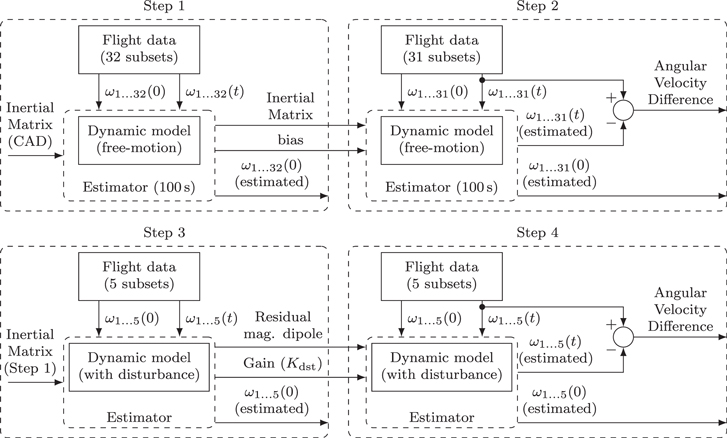
Figure 7. Attitude model identification and validation steps diagram.
Download figure:
Standard image High-resolution imageWe use the satellite dynamic model presented in Section 4.2 to determine the time window regarding PicSat open-loop data for which we can consider the external disturbances negligible. Isolating the derivative of the spacecraft angular velocity in Equation (1) gives

Equation (7) is the dynamic simulation form of Equation (1).
Considering the case in which magnetorquers are off ( T mtq = 0) and reaction wheels stopped ( H rw = 0), Equation (7) becomes

Omitting the sub and superscribed reference frames and taking the integration of Equation (8) between times ti and tf, we obtain
The first term in Equation (9) is the angular velocity of free motion, and depends only on the satellite initial velocity and its own gyroscopic torque:

In Equation (10), if  then ∥

The worst case for Equation (11) occurs when T dst is maximum and constant, that is,
Thus, the ratio between the free motion and the maximum disturbance in terms of norm of angular velocity is
In attitude modeling for closed-loop control, we may neglect disturbances of less than one tenth of the open-loop response amplitude, that is, ∥
Considering the suitable in-orbit data subsets for such evaluation, the lowest norm of the angular velocity was
Taking  from the PicSat
  , and
, and  estimated via the attitude dynamic model using initial values for parameters taken from satellite components data sheets, we find
  s−2. Thus
Therefore Step 1 must be applied to time windows up to 67.5 s. Since  is a very conservative estimation and a better value can be determined by iterating modeling results against in-orbit data, we will relax this constraint to 100 s allowing the use of more in-orbit data and improving model accuracy.
In order to measure
 in open-loop attitude response with magnetorquers off and reaction wheels stopped, analysis of in-orbit angular velocity data allowed us to identify 10 data stretches with at least 10 consecutive samples having the following lengths: 290, 680, 570, 300, 770, 600, 690, 750, 720 and 620 s. To carry out Steps 1 and 2, these stretches were divided into subsets of 100 s. When necessary to complete the last subset, data from the previous one was used. There were 63 subsets altogether.
5.1.1. Step 1—Satellite Dynamics Identification
For Step 1, 32 from the original 63 subsets were selected. An arbitrary rule was applied: the odd index subsets were chosen, that is, the first, the third, the fifth, and so on. PicSat inertia matrix, ADCS gyrometers' bias and initial velocity were optimized/estimated based on a nonlinear least squares approach using those subsets, that is, they were all free parameters of the optimization algorithm. Principal inertia moments varied from about 1% in X and Y axes to 10% in Z-axis comparing
In order to quantify the difference between in-orbit data and the identified attitude model, we employ the metric

where diff is a vector containing the ℓ2-norm of the angular velocity difference between in-orbit and modeled satellite angular velocity, N is the number of measurements acquired between ti and tf. As Equation (12) is a summation of modeling residues, its value increases with time for each velocity axis. More classical metrics would lead us to deal with in-orbit data noise filtering, which is an extra work without any big advantage in terms of modeling accuracy regarding closed-loop control.
Figure 8 shows the identification results for the angular velocity in terms of Equation (12). In this plot each dot is the result of summation of 100 s of ℓ2-norm data.

Figure 8. Step 1 results—summation of the ℓ2-norm of the difference between in-orbit and modeled satellite angular velocity for all subsets.
Download figure:
Standard image High-resolution imageThe average differences are distributed around the abscissa axis, indicating residual randomness. Summation of norm is typically around 7 × 10⁻³ rad s−1, which means that identification residuals are very small. We show them in more details in Step 2. Only for Z-axis, norm summation is as high as 2 × 10⁻² rad s−1, which is due to the gyrometer noise.
5.1.2. Step 2—Satellite Dynamics Validation
The validation was performed with the other 31 subsets. In this case, even indexes were used, that is, the second, the fourth, the sixth and so on. An example of result for one subset is shown in Figure 9.

Figure 9. Step 2 results for one subset.
Download figure:
Standard image High-resolution imageOne can see an excellent match between in-orbit and modeled angular velocity, except for Z-axis, which is not due to the dynamic model. Instead, it is due to high gyrometer noise. In this time frame (100 s), the satellite behaves as a rigid body in free motion. Thus, we have kinetic energy being exchanged among its three rotation axes, which means that angular velocities are coupled and are constrained by the rigid body dynamics. Thus, it is physically impossible to have Z-axis high-frequency velocity while X and Y axes move slowly. One can observe this behavior all around the subsets in Figure 8 as well. Therefore, for modeling and validation purposes, X and Y axes raw data are more reliable them Z-axis data. If we apply a low-pass filter matching the frequency domain of the satellite dynamics, they will be more consistently reliable. We have not designed and implemented such a filter, because a proper development requires detailed knowledge about the flight sensors while the raw data accuracy is already enough for dynamic modeling in terms of ADCS.
Figure 10 shows the validation results for the angular velocity in terms of Equation (12). In this plot each dot is the result of summation of 100 s of ℓ2-norm data. In other words, Figure 9 becomes three dots in Figure 10, one for each axis.

Figure 10. Step 2 results—summation of the ℓ2-norm of the difference between in-orbit and modeled satellite angular velocity for all subsets.
Download figure:
Standard image High-resolution imageAs for the identification results, the average differences appear to be random. This time, Figure 9 helps to understand what the amplitudes mean. The summation of the norm for the X-axis is 0.5 × 10⁻² rad s−1, for the Y-axis is 1 × 10⁻² rad s−1 and for the Z-axis is 2 × 10⁻² rad s−1. Therefore, 1 ×10⁻² rad s−1 or less indicates a really good match between real data and model.
5.1.3. Step 3—External Disturbances Identification
To accommodate uncertainties on the disturbance model parameters, and even data time stamping bias, a disturbance gain, Kdst, was introduced in Equation (2), leading to:

where the residual magnetic dipole ( m mag) will be also a degree of freedom, as long as it is the most important disturbance in the specific case of PicSat.
As in Step 1, to perform Step 3 we selected 5 subsets alternately from the original 10 ones. The subsets are now longer than 100 s. The validated inertia matrix and gyro bias are obtained from Step 2. As previously, the procedure to identify Kdst and m mag utilized a nonlinear least squares approach. The values obtained were
and

Figure 11 shows the identification results for the angular velocity.

Figure 11. Step 3 results—summation of the ℓ2-norm of the difference between in-orbit and modeled satellite angular velocity for all subsets.
Download figure:
Standard image High-resolution imageStep 3 utilizes a small number of subsets when compared to Steps 1 and 2. Another difference is that this time the duration is as long as 700 s. Even so, the summation of norm gives results in the order of 2 to 4 × 10⁻² rad s−1, which is remarkably low. Therefore, disturbances have been adequately modeled.
Feedback control can deal with disturbances which are unknown or known with some degree of accuracy. Step 3 results are sufficient for designing a compensator for PicSat.
5.1.4. Step 4—External Disturbances Validation
External disturbances validation was performed using the other 5 subsets. An example of result for one subset is shown in Figure 12.

Figure 12. Attitude disturbance model validation results for one subset.
Download figure:
Standard image High-resolution imageThere is an excellent match between in-orbit and modeled angular velocity even in the presence of external disturbances. The spectral density of differences is not concentrated in any specific frequency, which indicates that no systematic modeling error is present.
Figure 13 presents a zoom-in in the modeled external disturbances. The torque due to the residual magnetic dipole, T mag, is the most important for PicSat. It is partially a consequence of letting m mag as a free parameter and partially because, indeed, the residual magnetic dipole is typically the most relevant external disturbance torque for CubeSats. Nevertheless, any other choice would have produced a distortion in terms of disturbance weight and would not be appropriate. Figure 13 also shows that the torque due to the solar radiation pressure, T srp, is the less important.

Figure 13. Validated attitude disturbances (absolute torques) for Subset 1.
Download figure:
Standard image High-resolution imageIn Section 5.1, using theoretical and nominal values, we have determined that for time frames smaller than 100 s, the influence of the external disturbances would be ten times less than the free motion dynamics. To verify this premise, Figure 14 presents simulations comparing the presence and absence of disturbances in the satellite's dynamic model against in-orbit data. One can observe a clear increase in the modeling error after 150 s if disturbance is not taking into account in the model.

Figure 14. Comparison between presence and absence of disturbances over time—Subset 1. Real data and simulation with (w/) and without (s/) disturbances.
Download figure:
Standard image High-resolution imageMore precisely, when simulation reaches 200 s, the ratio between external torque and free motion reaches about 1/10. Figure 15 shows the ratio evolution regarding the time window. Such result is computed based on the validated model.

Figure 15. Disturbance to free motion ratio regarding time window.
Download figure:
Standard image High-resolution imageThe time window of 100 s adopted is consistent with negligible disturbance. The whole set of validation results for angular velocity is presented in Figure 16. As in the estimation results, the summation stays at very low values indicating the modeling accuracy achieved suffices for feedback control.

Figure 16. Step 4 results—summation of the ℓ2-norm of the difference between in-orbit and modeled satellite angular velocity for all subsets.
Download figure:
Standard image High-resolution image5.2. Orbit Propagation Identification and Validation
The orbital position of a satellite can be obtained by means of a GPS device on board the spacecraft, or by tracking radars on the ground. PicSat lacked either system. However, the U.S. Space Surveillance Network tracks all objects in Earth orbit (artificial satellites and debris) and maintains a cataloged database of them (Vallado 2013). Their data are published by the Joint Space Operations Center on the portal Space-Track.org 10 in a format called Two-Line Element (TLE).
To estimate its current position, the ODS has an embedded orbit propagator, 11 which receives the last available TLE from the ground station.
For a given object, the time between TLE updates is not regular. It can vary from a fraction of the orbit to several days. Figure 17 shows the histogram of the update time between the PicSat TLEs from 2018 January 12 through 2019 September 29.

Figure 17. Histogram of PicSat's TLEs updates available from 2018 January 12 through 2019 September 29.
Download figure:
Standard image High-resolution imageAltogether there were 1166 updates during this time span. The longest interval between TLEs was 30 orbits, equivalent to 47.4 hr and 75% of updates occurred in less than a 11 hr interval.
The published TLEs lack accuracy information. However, in Riesing (2015) the Planet CubeSats constellation Flock 1B was used to determine the accuracy of the TLEs of these spacecraft, once they were equipped with a GPS module. As with PicSat, they were 3Us CubeSats, launched from the ISS. Ten satellites were deployed during 2014 September and 634 TLE updates occurred during that time. The statistical error in position could be estimated with good statistical accuracy to be less than 2.01 km in 25% of cases (first quartile), less than 4.52 km in 50% of cases (median), and less than 10.60 km in 75% of cases (third quartile).
Although contact with PicSat was lost on 2018 March 20, TLEs will continue to be available until the satellite re-enters Earth's atmosphere. We performed the identification and validation of the simulator's orbital propagation using the available TLEs for PicSat and the statistical error obtained in Riesing (2015). For this purpose, the following procedure was carried out: using TLEs as initial conditions for the simulator, we propagate the states until the next available TLE, comparing them at the end. We repeat this process ranging from TLEs available between one orbit up to 16 orbits (i.e., about 1 day between two TLEs). The results of the propagation error are shown in Figure 18. The horizontal dashed lines represent the statistical errors obtained in Riesing (2015).

Figure 18. Evolution of the orbital propagation difference between TLEs and model according to the number of propagated orbits.
Download figure:
Standard image High-resolution imageModel error increases with the propagation time. After 15 orbits, the median error of the model is 7.1 km, which is a very small error considering that 648,047.7 km were covered, i.e., 1.1 × 10⁻⁷% propagation error in 15 orbits. For an observer on the ground, it is equivalent to  uncertainty in pointing toward the spacecraft. For payloads that do not demand very high accuracy orbit determination, such propagator accuracy is sufficient.
Based on this model, the predicted re-enter date for PicSat is 2022 December 24 03:44:34 (UTC).
6. ADCS De-tumbling Mode
PicSat was placed in orbit by a QuadPack CubeSat Deployer. Such deployers eject CubeSats by means of compressed springs that generate an initial angular velocity on the satellites. PicSat in-orbit data shows an initial velocity of 1.78 deg s−1.
After launch, the ADCS should be able to reduce the spacecraft angular velocity down to 0.2 deg s−1 (standard limit for proper working of the star tracker) and then pointing the target star with a maximum error of ±30'' rms.
The iADCS-100 system has five operation modes: Idle, Safe, Measurement, De-tumbling and Target Pointing. Only the last two modes are closed-loop controllers. The De-tumbling Mode stabilizes the satellite angular velocity, reducing it to the requirement and the Target Pointing Mode points the payload toward the target star within the required accuracy.
The De-tumbling Mode uses only magnetorquers as actuators, and the Target Pointing Mode uses reaction wheels for pointing the satellite and magnetorquers for desaturating reaction wheels. By reducing the angular velocity, the De-tumbling Mode allows image acquisition from the star tracker's Lost in Space Mode, which provides the line of sight, preparing the ADCS to switch to Target Pointing Mode.
The De-tumbling Mode uses the simplest closed-loop controller. The exact structure of the proprietary de-tumbling controller used by PicSat's ADCS is unknown. Nevertheless, the Interface Control Document furnished with iADCS-100 clearly states that a B-dot controller is used for de-tumbling with two possible working configurations: proportional gain and maximum gain. First presented by Stickler & Alfriend (1976), the B-dot technique follows the principle of gradually reducing the spacecraft's rotational kinetic energy with the aid of the Earth's magnetic field. The control law polarizes the magnetorquers in the opposite direction of the local magnetic field derivative,  , from where the technique's name is derived.
The control law is expressed by:

where A
m
m is the dipole moment and  is the controller gain (diagonal matrix), with
  .
.
6.1. De-tumbling Mode: Model Identification and In-orbit Data Validation
Figure 19 shows the PicSat angular velocity norm during the entire mission. Start and stop commands for de-tumbling mode are signaled with dashed and dotted vertical lines, respectively. Three of the occasions, where an effective reduction in angular velocity can be seen, are marked by numbers 1–3.

Figure 19. PicSat in-orbit angular velocity norm.
Download figure:
Standard image High-resolution imageConsidering the B-dot control structure,  gain and initial velocity were estimated in a way similar to the dynamics validation performed in Section 5.1, using Equation (12). Free parameters of the algorithm were the initial velocity and the controller gain. Once again, the procedure was performed using a nonlinear least squares method. Data stretch number 2 was used to do the estimation and data stretches number 1 and 3 were used for the validation. B-dot gain identification and validation results are shown in Figure 20.

Figure 20. De-tumbling control loop identification and validation results.
Download figure:
Standard image High-resolution imageThe identified controller (Equation (14)) presents a satisfactory result for the norm of angular velocities. This indicates that the kinetic energy reduction is achieved in a similar way for both flight and on-ground modeled controllers. However, if the in-orbit and modeled angular velocities are compared independently, axis by axis, the results are unsatisfactory, suggesting some inconsistency between them. Such an issue will be investigated and an advanced identification strategy as discussed in Romano & Pait (2017) will be applied to precisely determine what is missing in Equation (14).
7. Conclusions
In this paper, we have presented and validated a dynamic attitude and orbit propagation simulator for PicSat as well as its de-tumbling mode. High-precision dynamic models have been obtained for both attitude and orbit. Norm of the difference between the attitude model and in-orbit angular velocity has been determined to be typically lower than 0.04 rad s−1 over 700 s, while the orbit propagation is as accurate as ±500 m rms in one orbit. We have also properly simulated the de-tumbling angular velocity norm time series compared to in-orbit data.
Despite not having accomplished its astronomical goal, PicSat left us an enduring legacy: its platform data allowed us to perform a flight modeling that will be quite valuable for future missions. Such models are necessary for missions aiming to achieve high-performance pointing requirements (of the order of the arcsecond rms), as is the case of PicSat. They are also broadly suited for different mission phases, from spacecraft design to data exploitation.
Based on these models, many studies can be made for PicSat and any other CubeSat mission. Concerning PicSat, one can use the orbital propagator to apply orbital position correction to the available data as well as time stamping correction. The attitude dynamic model allows improving the two-stage control strategy, studying performance, observability, controllability, and system stability regarding nominal and degraded operation. It can be used to refine the control mode switch strategy and simulate issues as faced by PicSat to modify and improve on-board algorithms. For future missions, it can be also used for implementation of the ADCS embedded software in a re-programmable Real-Time Operation System, allowing for re-programmable in-flight control algorithms, a highly desirable improvement compared to PicSat's ADCS. It is essential to minimize the possibility of failure for both the platform and the payload, especially in satellites such as PicSat, whose pointing depends on both.
There is still a lot to learn from PicSat flight data. This work made it possible to prepare the bases for a more detailed understanding of its months of operation, which will allow a remarkable increase of reliability for upcoming CubeSat missions, both in the preparatory and exploitation mission phases. In this sense, we are already working in a C++ version of the models and control loop presented here to produce On-board In-Loop (OIL) and Hardware In the Loop (HIL) simulators. We are also going to study in more detail the de-tumbling mode.
The models obtained are a novel result and can be applied to any CubeSat in low Earth orbit, requiring only minor adaptation to each spacecraft. The decision whether to develop models to support ADCS simulators is linked to the mission criticality. They are indispensable in scientific missions, therefore scientific space research laboratories worldwide need to employ CubeSat dynamic modeling and control to succeed in the most challenging endeavors.
The PicSat satellite was designed, integrated and operated by Observatoire de Paris—PSL/CNRS. We would like to thank the students, engineers and researchers who made this project happen. The core team was Sylvestre Lacour, Vincent Lapeyrere, Mathias Nowak, Lester David, Antoine Crouzier, Guillaume Schworer and Maarten Roos.
The PicSat team were supported by the European Union under ERC grant 639248 LITHIUM.
Part of the work presented in this paper was supported by Fundação de Amparo à Pesquisa do Estado de São Paulo (FAPESP) under grants 2016/13750-6 and 2018/19585-2.
Appendix: Detailed Spacecraft and Disturbance Modeling
This appendix details the spacecraft and disturbance modeling.
A.1. Reference Frames
We start by clearly defining all necessary reference frames.
A.1.1. Earth-centered Inertial Reference Frame (ECI)
The ECI is denoted by {I}. It has its origin in the Earth's center of mass.  the X-axis unit vector is defined as the direction of the equinox of 2000 March, and represented by the Greek letter
  is taken at the north direction of the Earth's rotation axis and
  completes the right-handed Cartesian coordinate system.
A.1.2. Earth-centered Earth-fixed Reference Frame (ECEF)
The ECEF is a non-inertial frame denoted by {E}. It has its origin in the Earth's center of mass.  is defined as the direction of prime meridian,
  is taken at the north direction of the Earth's rotation axis and
  axis completes the right-handed Cartesian coordinate system and the (
 ,
,  )-plane forms the equatorial plane.
A.1.3. Spacecraft Reference Frame (SCRF)
The SCRF, denoted by {S}, has its origin O in the geometric center of the spacecraft,  axis is normal to the side that contains the antennas,
  axis is perpendicular to the satellite side and
  axis completes the right-handed coordinate system.
A.1.4. Attitude Control Reference Frame (ACRF)
The ACRF, denoted by {A}, has its origin is the spacecraft's center of mass CM,  axis being in the direction of the biggest moment of inertia,
  axis in the direction of the smaller moment of inertia and
  axis completes the right-handed coordinate system.
A.2. Transformation between Reference Frames
Reference frames can be related to each other by frame transformations.
A.2.1. Transformation between ECI and ECEF
Once the ECI and ECEF ( )-planes are coplanar, the rotation between them comes only from the Earth's rotation movement around the
  axis. Thus, the rotation matrix and its representation in quaternions are expressed by

and

where

where tU is the time in hours in UT1 scale, and
where T0 = dU/36525, and dU is the time in Julian days since J2000.0.
A.2.2. Transformation between SCRF and ACRF
The transformation of the spacecraft inertia matrix I sc, from SCRF or just {S} to ACRF or just {A}, is given by

where A I is the diagonal form of the spacecraft's inertia matrix, S I is the non-diagonal form of the spacecraft's inertia matrix and A Q S is the rotation matrix from {S} to {A}.
As shown in Curtis (2014), the matrix A I is formed, on the main diagonal, by the eigenvalues of S I and the matrix A Q S is formed by the respective eigenvectors of S I .
A.3. Attitude Representation
We can represent the satellite orientation by means of rotation matrices (also called direction cosine matrices), Euler angles, or quaternions. Rotation matrices are hard to read and computationally expensive. Euler angles are easy to read but present singularities and require the use of rotation matrices when transforming reference frames. Quaternions are hard to read and computationally inexpensive. Therefore, from now on we present results using Euler angles, and compute transformations using quaternions, which are preferable for embedded ACS (Sidi 1997; Curtis 2014).
The Euler angles are three angles describing the orientation of a rigid body with respect to a fixed coordinate system. Here they are expressed by (ϕ,
A quaternion can be expressed as:

where q0 is the scalar part and q is the vector or imaginary part (Wertz 1978).
By restricting the quaternion to be unitary,  , it is possible to relate it to the symmetrical Euler parameters.
The transformation between them using the 3-2-1 sequence is given by:
A.4. Satellite Kinematics
Concerning the satellite, kinematics describes its attitude and angular velocity time series without any concern about the torques that have created such movement.
Consider the spacecraft's Cartesian angular velocity described by

where

where
W
(
As
A.5. Satellite Dynamics
Attitude dynamics describes the angular velocity as a function of the applied torque T .
Most CubeSats can be considered rigid bodies, because they do not have moving parts and orbit control systems, which usually employ of propellants. Therefore, mass distribution remains constant over time. Although PicSat has a piezoelectric positioning system as part of the payload (Piezo-stage in Figure 4), it can be considered a rigid body for attitude dynamics modeling. As a result, rigid body dynamics properties and equations apply. Considering

where A
I
sc and A
A.6. Actuators
According to Table 1, PicSat is equipped with magnetic actuators and reaction wheels. Therefore, the torque due to actuators is given by Equation (A12)

where A T mtq is the total torque due to magnetorquers and A T rw is the total torque due to reaction wheels written in {A}.
We compute each of these torques in the next subsections.
A.6.1. Magnetorquers
In Low Earth Orbit (LEO), Earth's magnetic field intensity is not negligible (Wertz 1978). Its interaction with magnetorquers is capable of producing torque in the spacecraft. Physically, the actuator consists of a coil with a ferromagnetic core or air core. Therefore, it is possible, by Kirchhoff's Laws, to model it as a resistor and inductor series circuit. The magnetic moment is in the direction of the normal to the coil plane and the sense is given by the Right-Hand Rule. Its intensity is given by the Ampere's law. We neglect the demagnetization effect. The total intensity of the magnetic moment, mmtq, is the sum of the intensities of the magnetic moment generated by the coil and by the ferromagnetic core. In vector form, the magnetorquer's torque is given by Equation (A13)

where  is the magnetic moment of each dipole, and
B
the Earth's magnetic field.
is the magnetic moment of each dipole, and
B
the Earth's magnetic field.
A.6.2. Reaction Wheels
Reaction wheels (RW) allow more precise pointing control (Yost 2020). Considering
I
rw and

Only the first term of Equation (A14) ( ) can be used to control the spacecraft orientation. The second one (
 ) is a gyroscopic perturbation effect and it will be added to the satellite dynamics. Moreover, by action and reaction law, both terms must be negative. The final equation is:

The simplicity of Equation (A15) is suitable for PicSat modeling purposes. Nonlinear effects such as RW's imbalance (microvibrations), Coulomb friction and magnetic modeling, magnetorquer's demagnetization could be included in additional terms, depending on the requirements for each mission.
A.7. External Disturbances
This appendix section presents all relevant attitude and orbit external disturbances that PicSat faces during flight. Figure 21 presents a block diagram that summarizes them.

Figure 21. Attitude and orbital external disturbances diagram.
Download figure:
Standard image High-resolution image
A.7.1. Attitude Disturbances
References Wertz (1978), Vallado (2013) and Curtis (2014) were used to implement attitude disturbances dynamic equations.
Torque Due to Atmospheric Drag—In orbit, the surface of a spacecraft collides with atmospheric particles, creating a force that will produce a torque in relation to the satellite's center of mass. The aerodynamic force on a surface element dA, written with respect to {S}, is given by

where CD is the drag coefficient,  and
and  is the unit vector of the surface element.
The torque due to atmospheric drag is expressed in {S} as

where r dA is the position vector of the spacecraft's center of mass up to the surface element dA where the force d F d is being applied.
Atmospheric Model—Density (
Torque Due to Solar Radiation Pressure—The incidence of electromagnetic radiation on the spacecraft's surface generates disturbance torque. The main source of radiation is the direct radiation from the Sun. The intensity and direction of incidence, the shape and the optical properties of the satellite's surface are the main factors that influence the torque due to the solar radiation pressure.
Analogously to the torque due to atmospheric drag, we divide the spacecraft's surface into infinitesimal element and determine the force applied to each of them. Depending on the optical properties of the surface, radiation can be absorbed, reflected with the same incidence slope or reflected in a diffuse way. The differential radiation force due to each of these portions is given, respectively, by

and
where S is the radiation intensity, c is the speed of light, cra, crr and crd are, respectively, the absorbed, reflected and diffuse radiation coefficients, constrained to 0 ≤ cra + crr + crd ≤ 1.  and
and  are, respectively, the unit vector normal to the surface element and the unit vector parallel to the surface element and in the direction of radiation projection.
Thus the torque due to solar radiation pressure is given by
where r dA is the position vector of the spacecraft's center of mass up to the surface element dA where forces d F are being applied.
Torque Due to Gravity Gradient—The gravitational force depends on the distance to the object and its orientation. Therefore, each mass element of the spacecraft is subject to a different force. This force distribution produces torque when the mass of the satellite is not perfectly distributed. This phenomenon is referred to as the gravity gradient.
The torque due to the gravity gradient, A T gg, when is written with respect to {A}, is given by

where
Torque Due to Residual Magnetic Dipole—The interaction between the Earth's magnetic field and the spacecraft's magnetic dipole produces torque. This magnetic dipole may be desired, like the magnetic actuator presented in Appendix A.6.1, or undesired, like eddy current, hysteresis and other magnetic moments that may arise due to currents circulating in the electronic circuits of the spacecraft. Calling it the residual magnetic dipole, m mag, and using Equation (A13), the torque due to the residual magnetic dipole, T mag, is given by

in which B is the Earth's magnetic field and its modeling is treated below.
Model of the Earth's Magnetic Field—With the help of satellites and observatories, mathematical models of the Earth's magnetic field have been developed since the 1960s. The models mostly used by the scientific community are the International Geomagnetic Reference Field (IGRF) (Thébault et al. 2015), developed by the International Association of Geomagnetism and Aeronomy, and the World Magnetic Model (WMM) (Chulliat et al. 2015) developed by the United State National Geophysical Data Center and British Geological Survey. Both models are updated every five years and are publicly available. Software such as MATLAB and Simulink have these models integrated. This paper uses the IGRF-12 version from 2015.
A.7.2. Orbital Disturbances
References Vallado (2013), Curtis (2014) and Markley & Crassidis (2014) were used to implement orbital disturbances dynamic equations.
Acceleration Due to Atmospheric Drag—Atmospheric drag was initially explored in Appendix A.7.1. It interferes with the spacecraft's orbit by changing its acceleration. This disturbance in acceleration, a d, is given by

where msc is the mass of the spacecraft and F d is the drag force as shown in Equation (A16).
Acceleration Due to Solar Radiation Pressure—Analogously to the drag, the solar radiation pressure interferes in the attitude and also in the orbit of the satellite.
The disturbance a srp is given by

where msc is the mass of the spacecraft, F ra is the force due to the absorbed radiation (Equation (A18)), F rr is the force due to reflected radiation (Equation (A19)), and F rd is the force due to diffuse radiation (Equation (A20)).
Acceleration Due to Earth's Oblateness—The Earth's gravitational potential can be obtained through spherical harmonic expansion, generating an infinite series with associated Legendre polynomials.
To calculate the Earth's oblateness acceleration a ob, it is necessary to truncate the series to a certain degree m and order n, both parameters from Legandre polynomials. The most common implementation is performed with m = 0 and n = 2. However, as presented by Vallado (2013), for a high-fidelity mathematical model, it is necessary to consider truncation at least at m = n = 24.
The most complete gravitational model is the Earth Gravitational Model 2008 (EGM2008) published by the U.S. National Geospatial-Intelligence Agency which allows truncation up to degree 2190 and order 2159 (Pavlis et al. 2012). In this paper, EGM2008 was used and the simulations were performed with truncation at m = n = 70.
Acceleration Due to Third-Body—Kepler's Orbit takes into account the gravitational interaction between two bodies. Such a situation is often referred to as the Two-Body Problem. However, other celestial bodies, such as the Moon and the Sun, will also interact gravitationally with the spacecraft. This interaction can be considered as a disturbance and modeled as a three-body system. Applying Kepler's law and considering the Moon and the Sun as third-bodies, the acceleration is given by
where
Footnotes
- 4
- 5
- 6
- 7
- 8
- 9
The
CAD model version made available was prior to final assembly, without cables and connections. In addition, those values were omitted here for confidentiality reasons. - 10
- 11